Introductory Economic Models

What is a Model?

In microeconomics, a model is a simplified description of reality used to explain and predict economic phenomena. Models help economists focus on the most important aspects of a problem by abstracting away less relevant details.

• Purpose: To provide a framework for understanding how the world works.

• Testing: Economists use data to evaluate the accuracy of models.

• Limitation: Models are not exact representations of reality; they are tools for generating testable predictions.

Additional info: The image above illustrates how a simple paper airplane can serve as a model for a real airplane, capturing essential features while omitting unnecessary complexity.

Evidence-Based Economics

Economists use real-world data to test models and answer practical questions, such as the value of a college education. For example, the opportunity cost of attending college includes both tuition and foregone earnings.

• Example: Calculating the opportunity cost of college using tuition fees and potential earnings at minimum wage.

The Scientific Method in Economics

The scientific method (or empiricism) in economics involves two main steps:

1. Developing models that explain some part of the world.

2. Testing those models using data to see how closely the model matches observations.

Economists often use experiments and natural experiments to measure cause and effect.

Correlation and Causation

Understanding Correlation and Causality

It is crucial to distinguish between correlation (when two variables move together) and causation (when one variable directly affects another).

• Positive correlation: Both variables move in the same direction.

• Negative correlation: Variables move in opposite directions.

• Spurious correlation: Variables are statistically related but not causally connected.

Correlation does not imply causality due to:

• Omitted variables: Missing factors that influence both variables.

• Reverse causality: The direction of cause and effect is opposite to what is assumed.

Examples of Spurious Correlation

Spurious correlations are statistical relationships that do not reflect a true causal connection. These examples highlight the importance of careful interpretation of data.

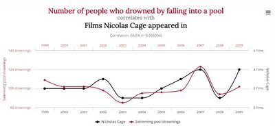
Additional info: The graphs above demonstrate how two unrelated variables can appear to move together, emphasizing that correlation alone is not evidence of causation.

Application: Returns to Education

Modeling the Returns to Education

Economists often use models to estimate the effect of education on earnings. A common assumption is that each additional year of education increases future earnings by a fixed percentage (e.g., 10%).

• Formula: If the base wage is $15 per hour, then after n additional years of education, the wage is:

• Example Calculation: After 4 years (a college degree):

• Percentage Increase: or 46.41% increase.

Testing the Model with Data

Real-world data can be used to test the predictions of the model. For example, average wages for different education levels in Canada show that college graduates earn about 43.5% more than high school graduates, which is close to the model's prediction.

Limitations of the Model

• Not everyone experiences the same wage increase with each year of education.

• The average can mask variation among individuals.

• Completing a degree may act as a signal of ability, not just increase productivity.

Statistical Measures: Mean and Median

Understanding Mean and Median

The mean (average) and median (middle value) are two common measures of central tendency in data analysis.

• Mean: Sum all values and divide by the number of observations.

• Median: The value that separates the higher half from the lower half of the data set.

Comparing the mean and median can reveal information about the distribution and inequality of data.

Appendix: Equations and Graphs

Graphing Linear Functions

Linear functions are commonly used in economics to represent relationships between variables. The general form is:

• A: Intercept (value of Y when X = 0)

• B: Slope (change in Y for a one-unit change in X)

Example with A = 5 and B = 2:

Application to Supply and Demand

In microeconomics, demand and supply functions are often written as:

where is quantity demanded, is quantity supplied, and is price.

Practice Problems

• Problem 1: Find two numbers whose sum is 385 and whose difference is 97.

• Problem 2: A fishing boat brings in cod and haddock. Cod sells for $2.00/lb, haddock for $1.50/lb. The total catch is 5,000 lbs and sells for $9,000. How many pounds of each were caught?