The Economic Analysis of Cost

Cost Concepts in Microeconomics

Understanding the different categories of costs is essential for analyzing firm behavior and production decisions in microeconomics. Costs are typically divided into fixed and variable costs, and their behavior is crucial for determining optimal output and pricing strategies.

• Fixed Costs: These are costs that do not change with the level of output. Examples include rent, salaries of permanent staff, and insurance. Fixed costs must be paid even if output is zero.

• Variable Costs: These costs vary directly with the level of output. Examples include raw materials, wages for hourly workers, and utilities used in production.

• Total Cost (TC): The sum of fixed and variable costs at any level of output. Formula:

• Average Cost (AC): The cost per unit of output, calculated as total cost divided by quantity produced. Formula:

• Marginal Cost (MC): The additional cost incurred by producing one more unit of output. Formula:

Example: If a factory has fixed costs of $1000 and variable costs of $500 for producing 100 units, then TC = $1500, AC = $15 per unit.

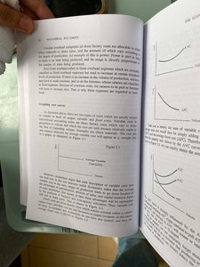
Graphing Cost Curves

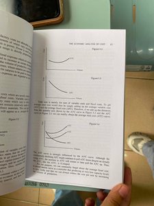
Cost curves are graphical representations of how costs change with output. The most common curves are Average Variable Cost (AVC), Average Total Cost (ATC), and Marginal Cost (MC). These curves help firms understand the relationship between output and costs, and are fundamental for decision-making.

• AVC Curve: Shows the average variable cost per unit at different output levels. Typically U-shaped due to economies and diseconomies of scale.

• ATC Curve: Shows the average total cost per unit. Also U-shaped, reflecting spreading of fixed costs and variable cost behavior.

• MC Curve: Shows the cost of producing one additional unit. Intersects AVC and ATC at their minimum points.

Example: As output increases, AVC and ATC initially decrease due to spreading fixed costs and increasing efficiency, then rise as diminishing returns set in.

C

Cost Functions and Mathematical Representation

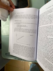
Cost functions express the relationship between cost and output mathematically. They are used to analyze and predict cost behavior for different production levels.

• Linear Cost Function: where 'a' is fixed cost and 'b' is variable cost per unit.

• Nonlinear Cost Function: Often used to model more complex cost behavior, such as increasing or decreasing marginal costs.

• Graphical Analysis: Cost functions can be plotted to visualize cost behavior and identify optimal production levels.

Example: If , then for Q = 10, TC = $150.

in setting prices, determining output levels, and maximizing profit. It also informs policy decisions and market structure analysis.

• Profit Maximization: Firms maximize profit where marginal cost equals marginal revenue ().

• Break-Even Analysis: Determines the output level at which total revenue equals total coApplications and Implications of Cost Analysis

  Cost analysis is fundamental for firmsst.

• Cost Minimization: Firms seek to produce at the lowest possible cost for a given output.

Example: A firm uses cost curves to decide whether to expand production or shut down in the short run.

Summary and Advanced Considerations

Advanced cost analysis includes consideration of opportunity costs, implicit costs, and the role of technology in reducing costs. Understanding these concepts is essential for comprehensive microeconomic analysis.

• Opportunity Cost: The value of the next best alternative foregone.

• Implicit Cost: Costs that do not involve direct payment but represent lost opportunities.

• Technological Change: Can shift cost curves downward, reducing costs for firms.

Example: Investing in new technology can lower variable costs and shift the ATC curve downward.