Modeling Motion

Introduction to Motion Models

In physics, motion is described using three main models: motion-dot (particle) models, graphs, and equations. These models help us visualize, analyze, and mathematically represent how objects move over time. Understanding these models is fundamental to kinematics, the study of motion.

• Motion-dot model (Particle Model): Visually shows the position of an object at equal time intervals, helping to identify patterns such as constant speed or acceleration.

• Graphs: Position-time and velocity-time graphs provide a visual representation of how position and velocity change over time.

• Equations: Mathematical relationships quantify motion, allowing for precise calculations.

Motion-dot Model (Particle Model)

Understanding Motion Diagrams

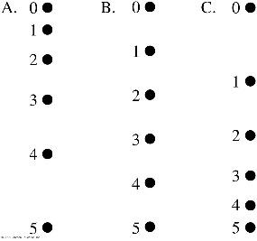
The motion-dot model represents an object's position at regular time intervals. The spacing between dots indicates the object's speed: equal spacing means constant speed, increasing spacing means acceleration, and decreasing spacing means deceleration.

• Constant Speed: Dots are evenly spaced.

• Acceleration: Dots get farther apart as time progresses.

• Deceleration: Dots get closer together as time progresses.

• Application: Used to analyze real-world scenarios such as a dust particle settling, a ball dropping, or a rocket landing.

Graphical Models of Motion

Position-Time Graphs

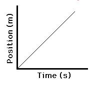
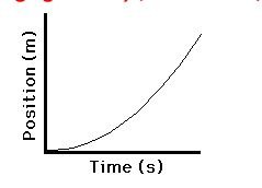
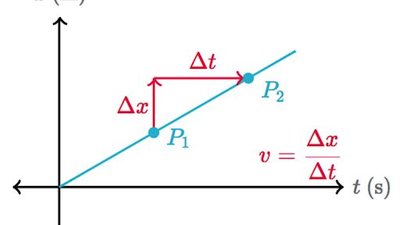
Position-time graphs plot an object's position against time. The slope of the graph represents the object's velocity. A straight line indicates constant velocity, while a curved line indicates changing velocity (acceleration).

• Constant Motion: Straight line with constant slope.

• Accelerated Motion: Curved line with increasing slope.

• Interpretation: The steeper the slope, the faster the object moves.

Velocity-Time Graphs

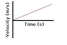
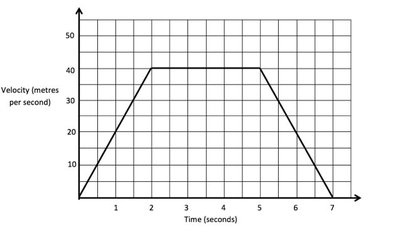
Velocity-time graphs show how an object's velocity changes over time. A flat line indicates constant velocity, while a sloped line indicates acceleration or deceleration.

• Constant Velocity: Flat horizontal line.

• Changing Velocity: Sloped line (upward for acceleration, downward for deceleration).

Mathematical Models of Motion

Equations for Average Velocity

Mathematical equations allow us to calculate average velocity and displacement. The average velocity is the slope of the position-time graph and is given by:

• Average Velocity Formula:

• Displacement:

• Distance: Total length traveled, always positive.

Example: Echo in the Grand Canyon

To find the depth of the Grand Canyon using the time for an echo and the speed of sound, use the formula:

• Distance Formula:

• Application: The time measured is for the sound to travel down and back, so divide by 2 for the one-way distance.

Additional info: The Grand Canyon image is not directly relevant to the calculation, so it is not included.

Math Review and Vocabulary

Key Terms in Kinematics

Understanding the vocabulary is essential for describing motion:

• Position: Location relative to an origin, can be positive or negative.

• Displacement: Change in position, can be positive or negative.

• Distance: Total space covered, always positive.

• Speed: Distance divided by time, direction independent.

• Velocity: Displacement divided by time, direction included.

• Scalar: Measurement with magnitude only (e.g., speed, distance).

• Vector: Measurement with magnitude and direction (e.g., velocity, displacement).

• Acceleration: Change in velocity over time.

Instantaneous vs. Average Velocity

Comparing Instantaneous and Average Values

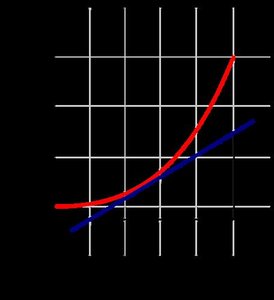
Instantaneous velocity is the slope of the position-time graph at a specific instant, often found using a tangent line. Average velocity is the slope between two points (secant line) and is calculated over a time interval.

• Instantaneous Velocity:

• Average Velocity:

Average Speed and Velocity Calculations

Solving for Average Values

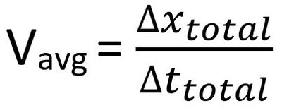
Average speed and velocity can be calculated for trips with varying speeds or distances. The formula is:

• Average Velocity Formula:

• Application: Use total displacement and total time for velocity; use total distance and total time for speed.

Area Under the Graph

Displacement from Velocity-Time Graphs

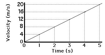
The area under a velocity-time graph represents the displacement of the object. This is because:

• Relationship: , so

• Interpretation: The area under the curve gives the total change in position.

Change in Velocity from Acceleration-Time Graphs

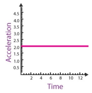
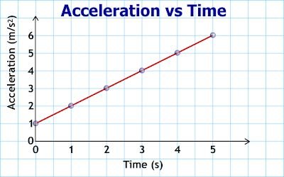
The area under an acceleration-time graph gives the change in velocity:

• Relationship: , so

• Interpretation: The area under the curve gives the total change in velocity.

Summary Table: Scalar vs. Vector Quantities

Conclusion

Modeling motion is a foundational skill in physics with algebra. By mastering motion-dot models, graphs, and equations, students can analyze and predict the behavior of moving objects. Understanding the relationships between position, velocity, and acceleration is essential for further study in kinematics and dynamics.