Functions and Graphs

Plotting Points in the Rectangular Coordinate System

The rectangular coordinate system is used to visually represent ordered pairs and relationships between variables. Each point is defined by an ordered pair (x, y), where x is the horizontal coordinate and y is the vertical coordinate. The origin is the point (0, 0), and the axes divide the plane into four quadrants.

• Ordered Pair: (x, y) represents a point where x is the horizontal position and y is the vertical position.

• Quadrants: The plane is divided into four regions by the x- and y-axes.

• Plotting Points: Move from the origin according to the values of x and y.

Example: Plot the points A(-3, 5), B(2, -4), C(5, 0), D(-5, -3), E(0, 4), and F(0, 0).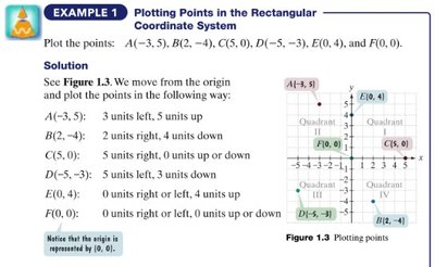

Graphs of Equations and Functions

A graph of an equation in two variables is the set of all points whose coordinates satisfy the equation. Functions are special relations where each input (x) corresponds to exactly one output (y).

• Function: A relation in which each input value leads to exactly one output value.

• Graph: The visual representation of all solutions to the equation.

Example: The graph below shows a function with varying behavior across its domain.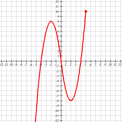

Evaluating Functions Using Tables

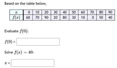
Tables can be used to evaluate function values and solve for inputs given outputs. This is useful for discrete data and for understanding the relationship between variables.

• Evaluate f(0): Find the output when x = 0.

• Solve f(x) = 40: Find the input(s) x for which the output is 40.

Identifying Domain and Range

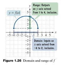
The domain of a function is the set of all possible input values (x), and the range is the set of all possible output values (y). These can be determined from graphs, tables, or equations.

• Domain: All x-values for which the function is defined.

• Range: All y-values that the function can produce.

Example: The domain and range can be visualized on a graph.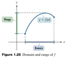

Intercepts of Functions

Intercepts are points where the graph crosses the axes. The x-intercept is where y = 0, and the y-intercept is where x = 0.

• x-intercept: Set y = 0 and solve for x.

• y-intercept: Set x = 0 and solve for y.

Example: The graph below shows intercepts clearly marked.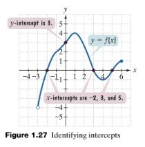

Increasing, Decreasing, and Constant Functions

A function can be classified as increasing, decreasing, or constant over intervals. These properties describe how the output changes as the input increases.

• Increasing: f(x) increases as x increases.

• Decreasing: f(x) decreases as x increases.

• Constant: f(x) remains the same as x increases.

Relative and Absolute Extrema

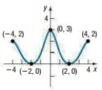
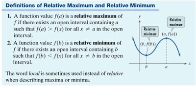
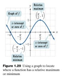
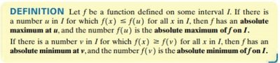
Functions may have relative maxima and minima (local high and low points), as well as absolute maxima and minima (highest and lowest values over the entire domain).

• Relative Maximum: f(a) is greater than nearby values.

• Relative Minimum: f(b) is less than nearby values.

• Absolute Maximum: Highest value of f(x) over the domain.

• Absolute Minimum: Lowest value of f(x) over the domain.

Symmetry in Functions

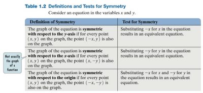
Graphs may exhibit symmetry with respect to the y-axis, x-axis, or origin. Symmetry can be tested algebraically by substituting variables.

• Y-axis Symmetry: Replace x with -x; if unchanged, symmetric about y-axis.

• X-axis Symmetry: Replace y with -y; if unchanged, symmetric about x-axis.

• Origin Symmetry: Replace x with -x and y with -y; if unchanged, symmetric about origin.

Even and Odd Functions

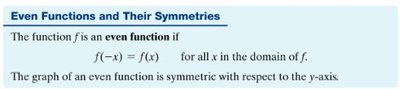
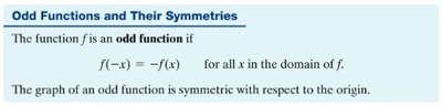
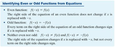
Even and odd functions have specific symmetry properties. An even function satisfies and is symmetric about the y-axis. An odd function satisfies and is symmetric about the origin.

• Even Function:

• Odd Function:

Difference Quotient

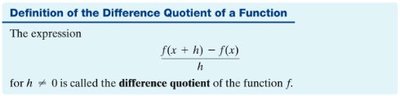
The difference quotient is a fundamental concept for understanding rates of change and is used extensively in calculus. It is defined as:

• Difference Quotient: , where

Linear Functions and Slope

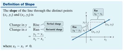
Linear functions are characterized by a constant rate of change, called the slope. The slope measures the steepness and direction of a line.

• Slope Formula:

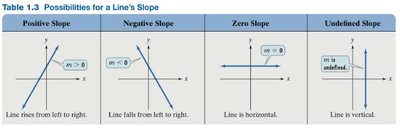
• Positive Slope: Line rises from left to right.

• Negative Slope: Line falls from left to right.

• Zero Slope: Line is horizontal.

• Undefined Slope: Line is vertical.

Equations of Lines

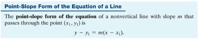
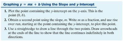
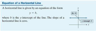
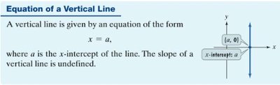
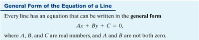
Lines can be represented in several forms: point-slope, slope-intercept, horizontal, vertical, and general form.

• Point-Slope Form:

• Slope-Intercept Form:

• Horizontal Line:

• Vertical Line:

• General Form:

Graphing Linear Equations Using Intercepts

Linear equations can be graphed efficiently by finding their x- and y-intercepts and drawing a line through these points.

• x-intercept: Set y = 0 and solve for x.

• y-intercept: Set x = 0 and solve for y.

Parallel and Perpendicular Lines

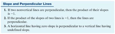
Parallel lines have equal slopes, while perpendicular lines have slopes that are negative reciprocals of each other.

• Parallel Lines: Slopes are equal.

• Perpendicular Lines: Product of slopes is -1.

Average Rate of Change

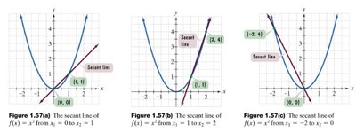
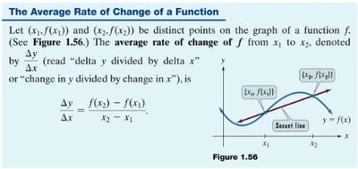
The average rate of change of a function between two points measures how the output changes per unit increase in input. It is analogous to the slope of the secant line between two points.

• Average Rate of Change:

Applications of Rate of Change

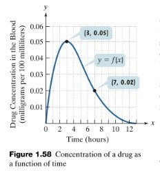
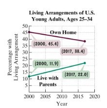
Rate of change is used in real-world contexts, such as population growth, velocity, and concentration of substances over time.

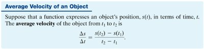
• Average Velocity: