뒤로
뒤로Chapter 3: Numerical Descriptive Measures in Introductory Statistics
스터디 가이드 - 스마트 노트
 자료에 맞춘 맞춤형 노트, 핵심 정의, 예시, 맥락을 확장해 제공합니다.
3.1 Measures of Central Tendency for Ungrouped Data
Definition and Importance
Measures of central tendency are statistical values that describe the center or typical value of a data set. The three main measures are the mean, median, and mode. These measures help summarize large data sets with a single representative value.

Mean
The mean (or average) is calculated by dividing the sum of all values by the number of values in the data set. It is sensitive to every value, including outliers.
Population Mean:
Sample Mean:
Where is the sum of all values, is the population size, is the sample size, is the population mean, and is the sample mean.
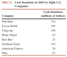
Example: Table 3.1 shows cash donations by eight U.S. companies in 2010. The mean donation is calculated by summing all donations and dividing by 8.
Median
The median is the value of the middle term in a data set arranged in increasing order. If the number of values is odd, the median is the middle value; if even, it is the average of the two middle values. The median is less affected by outliers than the mean.
Steps to Find the Median:
Rank the data in increasing order.
Identify the middle term(s).
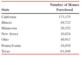
Example: Table 3.2 lists the number of homes foreclosed in seven states in 2010. The median is the fourth value when the data is ordered.

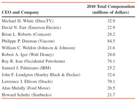
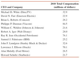
Example: Table 3.3 shows the total compensation of 12 highest-paid CEOs in 2010. The median is the average of the 6th and 7th values in the ordered list.

Mode
The mode is the value that occurs most frequently in a data set. A data set may have no mode, one mode (unimodal), two modes (bimodal), or more than two modes (multimodal). The mode can be used for both quantitative and qualitative data.
Unimodal: One mode
Bimodal: Two modes
Multimodal: More than two modes
Relationships Among the Mean, Median, and Mode
The relationship among mean, median, and mode depends on the shape of the data distribution:
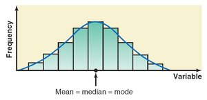
Symmetric Distribution: Mean = Median = Mode
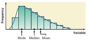
Right-Skewed Distribution: Mean > Median > Mode
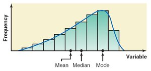
Left-Skewed Distribution: Mean < Median < Mode
3.2 Measures of Dispersion for Ungrouped Data

Range
The range is the difference between the largest and smallest values in a data set. It is a simple measure of dispersion but is highly sensitive to outliers.
Formula:
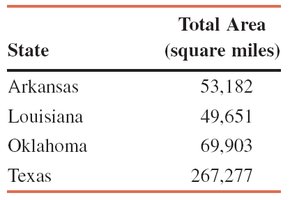
Example: Table 3.4 shows the total area of four western South-Central states. The range is calculated as the difference between the largest and smallest area values.
Variance and Standard Deviation
The variance and standard deviation measure how much the values in a data set deviate from the mean. The standard deviation is the square root of the variance and is the most commonly used measure of dispersion.
Population Variance:
Sample Variance:
Population Standard Deviation:
Sample Standard Deviation:
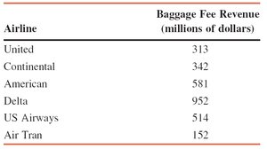
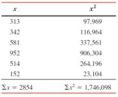
Example: Table shows baggage fee revenues for six airlines and the calculation of and for variance and standard deviation.
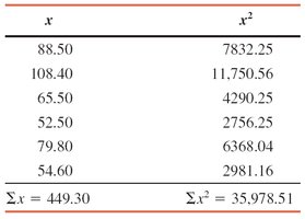
Example: Table shows earnings for six employees and the calculation of and .
3.3 Mean, Variance, and Standard Deviation for Grouped Data

Mean for Grouped Data
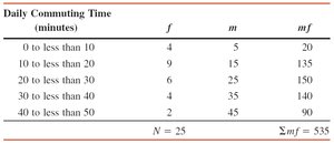
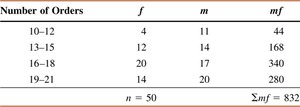
For grouped data, the mean is calculated using the midpoints of the classes and their frequencies.
Population Mean:
Sample Mean:
Where is the class midpoint and is the class frequency.
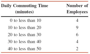
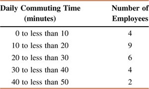
Example: Table 3.8 shows the frequency distribution of daily commuting times for 25 employees.
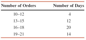
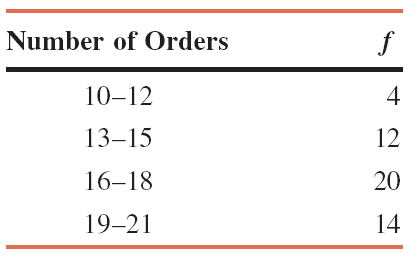
Example: Table 3.10 shows the frequency distribution of the number of orders received each day over 50 days.
Variance and Standard Deviation for Grouped Data
Population Variance:
Sample Variance:
Short-cut formulas are also available for computational efficiency.
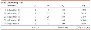
Example: Table shows the calculation for variance and standard deviation of daily commuting times.
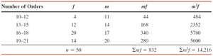
Example: Table shows the calculation for variance and standard deviation of number of orders received.
Use of Standard Deviation
Chebyshev’s Theorem
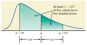
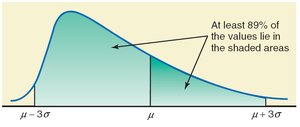
Chebyshev’s theorem states that for any data set (regardless of shape), at least of the data values lie within standard deviations of the mean, where .
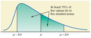
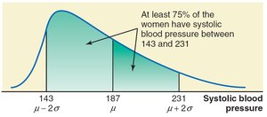
Example: For a mean of 187 and standard deviation of 22, at least 75% of values lie between 143 and 231.

Empirical Rule
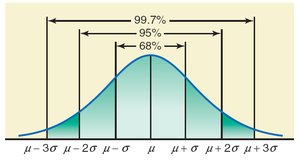
For bell-shaped (normal) distributions:
About 68% of values lie within 1 standard deviation of the mean
About 95% within 2 standard deviations
About 99.7% within 3 standard deviations
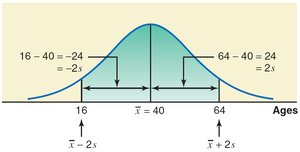
Example: For a mean age of 40 and standard deviation of 12, about 95% of people are between 16 and 64 years old.
Measures of Position
Quartiles and Interquartile Range (IQR)
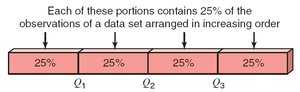
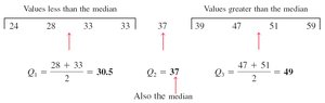
Quartiles divide a ranked data set into four equal parts. The interquartile range (IQR) is the difference between the third and first quartiles and measures the spread of the middle 50% of the data.
Formula:
Example: Table 3.3 (CEO compensation) is used to find quartiles and IQR.
Example: Quartile calculation for employee ages.
Percentiles and Percentile Rank
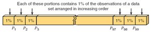
Percentiles divide a data set into 100 equal parts. The k-th percentile is the value below which k% of the data fall. The percentile rank of a value is the percentage of values in the data set that are less than that value.
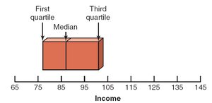
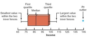
Box-and-Whisker Plot
A box-and-whisker plot visually displays the center, spread, and skewness of a data set using the median, quartiles, and extremes (excluding outliers).