Chi-Square Tests

Types of Pearson’s Chi-Square Tests

The Pearson’s chi-square test is a statistical method used to analyze categorical data. There are two main types:

• Chi-square goodness of fit test: Tests whether the observed frequency distribution of a single categorical variable matches an expected distribution.

• Chi-square test of independence: Tests whether two categorical variables are independent or associated.

Chi-square is often denoted as .

Goodness of Fit Test Example: Gold Lotto

To determine if the Gold Lotto is fair, we compare the observed frequencies of outcomes to the expected frequencies. The calculation involves:

• Listing all possible outcomes and their observed frequencies.

• Calculating the difference between observed and expected frequencies.

• Squaring the differences and dividing by the expected frequency for each outcome.

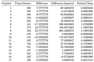
The sum of the Partial ChiSq column gives the test statistic .

Interpreting the Test Statistic

• Degrees of freedom (DF) = number of categories - 1

• Significance level (α) is typically 0.05

• Compare the calculated test statistic to the critical value from the chi-square distribution table

If the test statistic is less than the critical value, do not reject the null hypothesis (). If it is greater, reject $H_0$.

Chi-Square Test of Independence Example

To test if students' favorite subjects are associated with their grade levels, a contingency table is constructed and expected values are calculated. The test statistic is computed as:

• , where is observed frequency and is expected frequency.

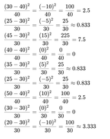
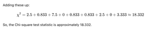
Degrees of freedom: , where is the number of rows and is the number of columns.

Compare the calculated statistic to the critical value (e.g., 9.488 for df=4, α=0.05). If the statistic exceeds the critical value, reject .

One-Sample Proportion Z-Test

Purpose and Formula

The one-sample proportion z-test is used to determine if the proportion of successes in a sample is significantly different from a known or hypothesized population proportion.

The test statistic is calculated as:

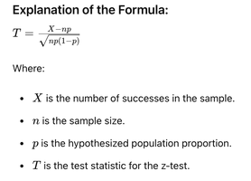
• X: Number of successes in the sample

• n: Sample size

• p: Hypothesized population proportion

• T: Test statistic

Critical Values and Decision Rules

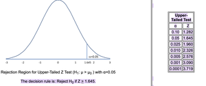
For a one-tailed test at α = 0.05, the critical value is approximately 1.645. If the calculated test statistic exceeds this value, reject .

One-Sample Z-Test for a Mean

Purpose and Assumptions

The one-sample Z-test for a mean is used to determine if the mean of a sample is significantly different from a known or hypothesized population mean. The population standard deviation () must be known, and the data should be approximately normally distributed.

Test Statistic Formula

The test statistic is calculated as:

• : Sample mean

• : Population mean

• : Population standard deviation

• n: Sample size

Critical Values and Rejection Regions

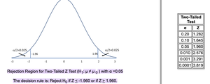
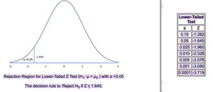
For a left-tailed test at α = 0.05, the critical value is -1.645. For a two-tailed test at α = 0.05, the critical values are ±1.96.

Example Calculation

Suppose a sample mean is 66, population mean is 65, population standard deviation is 3, and sample size is 50:

Since 2.36 > 1.96, we reject the null hypothesis at α = 0.05.

Interpreting Results

• If the test statistic falls in the rejection region, reject .

• If the test statistic does not fall in the rejection region, do not reject .

• Alternatively, compare the p-value to α: if p-value < α, reject .

Summary Table: Comparison of Tests