Describing, Exploring, and Comparing Data

Measures of Center

Measures of center are statistical values that describe the central point of a data set. The most common measures include the mean, median, and mode, each providing a different perspective on the data's central tendency.

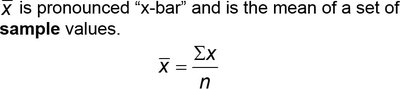
• Mean (Arithmetic Mean): The mean is calculated by summing all data values and dividing by the number of values. It is denoted as \( \bar{x} \) for samples and \( \mu \) for populations.

• Median: The median is the middle value when data are arranged in order. If the number of values is odd, it is the central value; if even, it is the mean of the two central values.

• Mode: The mode is the value(s) that occur most frequently in the data set. A set may have no mode, one mode, or multiple modes (bimodal or multimodal).

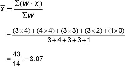
• Weighted Mean: Used when data values have different weights. The weighted mean is calculated as \( \bar{x} = \frac{\sum (w \cdot x)}{\sum w} \).

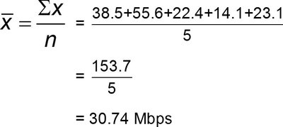
Example: Calculating the mean for sample data speeds:

Example: Calculating a weighted mean (grade-point average):

Measures of Variation

Measures of variation describe the spread or dispersion of data values. Common measures include range, standard deviation, and variance.

• Range: The difference between the maximum and minimum values in the data set.

• Standard Deviation: Indicates how much data values deviate from the mean. For a sample, it is denoted by s; for a population, by σ.

• Variance: The square of the standard deviation. Sample variance is s², population variance is σ².

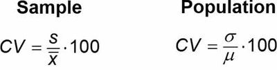
• Coefficient of Variation (CV): Expresses standard deviation as a percentage of the mean, useful for comparing variability between different data sets.

Standard Deviation Formulas:

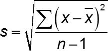
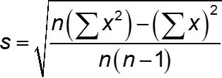
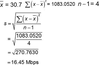
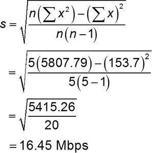
Example: Calculating sample standard deviation:

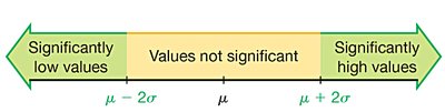
Range Rule of Thumb: Most values lie within 2 standard deviations of the mean. Significantly low values are at or below \( \mu - 2\sigma \), and significantly high values are at or above \( \mu + 2\sigma \).

Population Standard Deviation Formula:

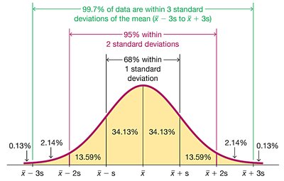
Empirical Rule: For bell-shaped distributions:

• 68% of values within 1 standard deviation

• 95% within 2 standard deviations

• 99.7% within 3 standard deviations

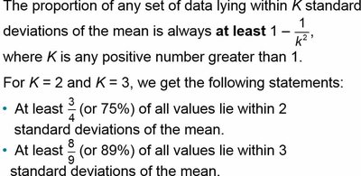
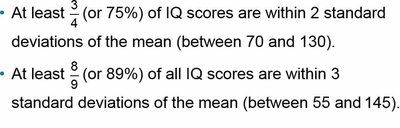
Chebyshev’s Theorem: Applies to any data set, not just bell-shaped distributions. At least \( 1 - \frac{1}{k^2} \) of values lie within k standard deviations of the mean.

Coefficient of Variation Formulas:

Measures of Relative Standing and Boxplots

Measures of relative standing indicate the position of a data value within a data set. Common measures include z scores, percentiles, quartiles, and boxplots.

• z Score: Indicates how many standard deviations a value is from the mean. Calculated as \( z = \frac{x - \bar{x}}{s} \) for samples or \( z = \frac{x - \mu}{\sigma} \) for populations.

• Percentiles: Divide data into 100 groups, each containing about 1% of the values.

• Quartiles: Divide data into four groups, each containing about 25% of the values. Q1 is the 25th percentile, Q2 is the median (50th percentile), Q3 is the 75th percentile.

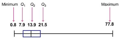
• 5-Number Summary: Consists of the minimum, Q1, median (Q2), Q3, and maximum.

• Boxplot: A graphical representation of the 5-number summary.

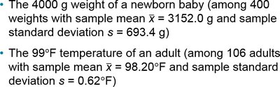
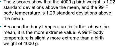
Example: Comparing z scores for baby weight and adult temperature:

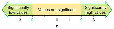
Example: Identifying significant values using z scores:

Percentile Calculation Procedure:

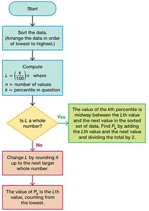
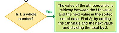
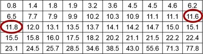
Example: Finding the 40th percentile in a sorted data set:

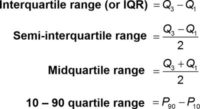
Quartile and Interquartile Range Formulas:

Example: Finding the 5-number summary:

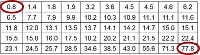
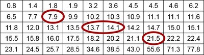
Example: Constructing a boxplot: