Describing Data Numerically

Measures of Central Tendency

Measures of central tendency summarize a data set with a single value that represents the center of the distribution. The most common measures are mean, median, and mode.

• Mean: The arithmetic average of the data values. For a population, the mean is denoted by μ and calculated as , where N is the population size. For a sample, the mean is denoted by x̅ and calculated as , where n is the sample size.

• Median: The middle value when the data are ordered. If n is odd, the median is the middle value; if n is even, it is the mean of the two middle values.

• Mode: The value that occurs most frequently in the data set. A set may have one mode, more than one mode (bimodal, multimodal), or no mode.

Outliers are values that are much higher or lower than the rest of the data. Outliers can strongly affect the mean, but have less effect on the median and mode.

Shapes of Distributions

The shape of a distribution describes how data values are spread. Common shapes include symmetric, uniform, and skewed distributions.

• Symmetric Distribution: Both sides are mirror images. Mean ≈ Median.

• Uniform Distribution: All classes have equal frequencies. Also symmetric.

• Skewed Distribution: One tail is longer than the other. Skewed left means the tail extends to the left; skewed right means the tail extends to the right. The mean is pulled toward the longer tail.

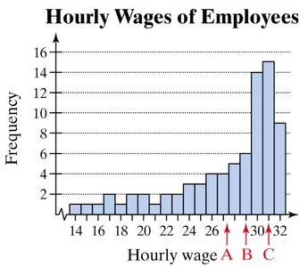
Example: The histogram below shows hourly wages of employees. Points A, B, and C are marked on the horizontal axis. The distribution is skewed left, with most values concentrated at higher wages. Among A, B, and C, the mean is pulled toward the lower values (A), the median is near the center (B), and the mode is at the highest frequency (C).

Measures of Variation

Range

The range measures the spread from the smallest to the largest data value. It is calculated as:

Variance and Standard Deviation

Variance and standard deviation measure how much the data values deviate from the mean.

• Population Variance:

• Population Standard Deviation:

• Sample Variance:

• Sample Standard Deviation:

Standard deviation indicates how spread out the data are from the mean. A small standard deviation means data are clustered near the mean; a large standard deviation means data are more spread out.

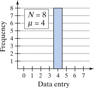
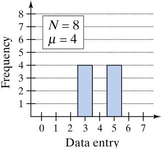
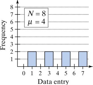
Example: Compare the standard deviations of the three data sets below. The first set has all values equal (standard deviation is zero), the second set has two groups (moderate spread), and the third set is uniformly spread (largest standard deviation).

Bell-Shaped Distributions and the Empirical Rule

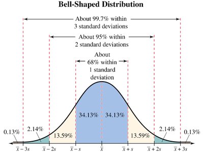
A bell-shaped distribution is symmetric about its mean, with most values concentrated near the center. The Empirical Rule states:

• About 68% of data lie within 1 standard deviation of the mean ()

• About 95% within 2 standard deviations ()

• About 99.7% within 3 standard deviations ()

Chebyshev’s Theorem

Chebyshev’s Theorem applies to any distribution, not just bell-shaped. It states that at least of the data lie within k standard deviations of the mean, for .

• For : At least 75% of data within 2 standard deviations.

• For : At least 88.9% within 3 standard deviations.

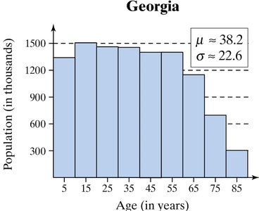
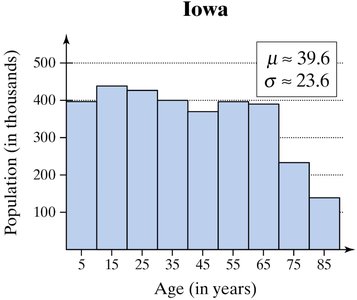
Example: The age distributions for Georgia and Iowa are shown below. Both have similar means and standard deviations. Using Chebyshev’s Theorem, an age of 90 is more than two standard deviations above the mean, so it is considered unusual for both states.

Measures of Position

Quartiles and Interquartile Range (IQR)

Quartiles divide an ordered data set into four equal parts:

• Q1: First quartile (25% below)

• Q2: Second quartile (median, 50% below)

• Q3: Third quartile (75% below)

The interquartile range (IQR) measures the spread of the middle 50% of the data: .

Outliers are values below or above .

Percentiles

A percentile indicates the percentage of data values less than a given value. The 50th percentile is the median.

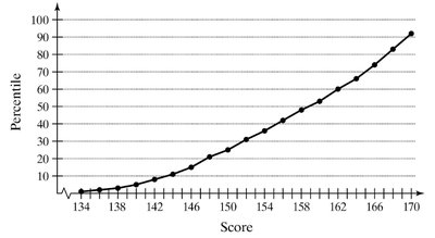
Example: The ogive below shows the cumulative frequency distribution of scores. The 50th percentile corresponds to the score where the cumulative frequency reaches 50%. The 80th percentile is where it reaches 80%. To find the percentile for a score of 162, locate 162 on the horizontal axis and read the corresponding percentile.

Standard Scores (z-Scores)

A z-score measures how many standard deviations a value is from the mean:

• z > 0: Value is above the mean

• z < 0: Value is below the mean

• z = 0: Value equals the mean

Values with |z| ≥ 2 are usually considered unusual; |z| ≥ 3 are very unusual.

Summary Table: Variance and Standard Deviation

Key Takeaways

• Central tendency measures (mean, median, mode) summarize the center of a data set.

• Variation measures (range, variance, standard deviation) describe the spread of data.

• Position measures (quartiles, percentiles, z-scores) locate values within the data set.

• Understanding the shape of a distribution helps interpret statistical results and identify outliers.