 뒤로
뒤로Normal Distribution and Sampling Distribution of Means: Study Notes
스터디 가이드 - 스마트 노트
 자료에 맞춘 맞춤형 노트, 핵심 정의, 예시, 맥락을 확장해 제공합니다.
Normal Distribution and Sampling Distribution of Means
Probability Density Function
The probability density function (PDF) is a fundamental concept in statistics used to compute probabilities for continuous random variables. It possesses two essential properties:
Non-negativity: The graph of the PDF must lie on or above the horizontal axis.
Total Area: The area under the graph must equal 1, representing the total probability.
Example: The normal distribution is a common example of a probability density function.
Normal Distribution
The normal distribution is a continuous probability distribution characterized by its bell-shaped and symmetric curve. It is also known as the Gaussian Distribution, named after Carl Gauss, and is widely used to model natural phenomena.
Notation: Normal distributions are denoted as N(μ, σ) or N(μ, σ2), where μ is the mean and σ is the standard deviation.
Range: The variable x ranges from −∞ to +∞.
Parameters: The distribution is fully described by its mean (μ) and standard deviation (σ).
Example: N(20, 3) or N(20, 32) represents a normal distribution with mean 20 and standard deviation 3.
Features of the Normal Curve
The normal curve exhibits several important features:
Bell-shaped: The curve is highest at the mean and symmetric about a vertical line through μ.
Central tendency: The mean, median, and mode are approximately equal (μ ≅ median ≅ mode).
Asymptotic: The curve approaches but never touches the horizontal axis.
Spread: As σ increases, the curve spreads out; as σ decreases, it becomes more peaked around μ.
Example: Curves with the same mean but different standard deviations will have different spreads.
Normal Distribution Function
The mathematical formula for the normal distribution is:
Where μ is the population mean and σ is the population standard deviation.
Example: A curve with μ = 2 and σ = 0.25 is more peaked than one with μ = 3 and σ = 0.5.
Normal Probability and Area Under the Curve
The area under the normal curve within a given interval represents the probability that a measurement will fall within that interval. The total area under the curve is 1, and the data is equally distributed on each side of the mean:
50% of the data lies to the left of μ
50% of the data lies to the right of μ
Identifying Normal Data
There are several methods to determine if a dataset follows a normal distribution:
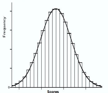
Histogram: A normal distribution's histogram should be roughly bell-shaped.
Outliers: A normal distribution should have no more than one outlier.
Quantile Plot (QQ Plot): If the data points lie close to a straight line, the data is approximately normal.
Example: The histogram below shows a bell-shaped distribution, indicating normality.
Empirical Rule (68-95-99.7 Rule)
The empirical rule describes the proportion of data within certain standard deviations of the mean in a normal distribution:
About 68% of the area is within one standard deviation (μ ± σ)
About 95% of the area is within two standard deviations (μ ± 2σ)
About 99.7% of the area is within three standard deviations (μ ± 3σ)
This rule is useful for quickly estimating probabilities and identifying outliers in normally distributed data.
