Organizing and Summarizing Data

Visualizing Qualitative vs. Quantitative Data

Visualizing data is a fundamental step in statistics, allowing us to understand patterns, distributions, and relationships within datasets. The choice of graph depends on whether the data is qualitative (categorical) or quantitative (numerical).

• Qualitative (Categorical) Data: Data that represents categories or labels, such as eye color or nationality.

• Quantitative Data: Data that represents numerical values, such as test scores or heights.

Graphs for Qualitative Data

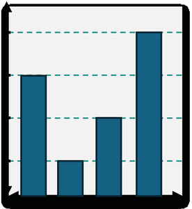
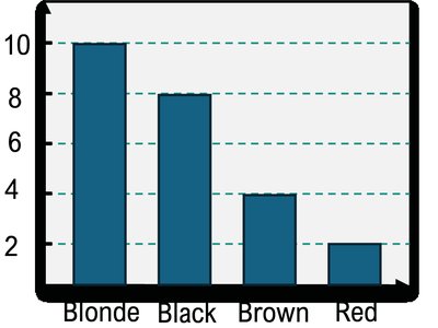
• Bar Chart: Displays frequencies for each category using bars. The height of each bar represents the frequency of the category.

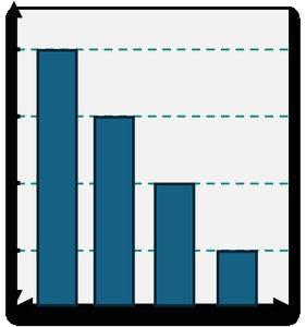
• Pareto Chart: A bar chart with bars arranged in descending order of frequency.

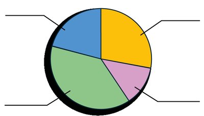
• Pie Chart: Shows the proportion of each category as a slice of a circle.

Graphs for Quantitative Data

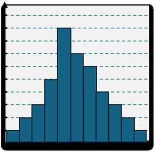
• Histogram: Uses adjacent bars to show frequencies for ranges (classes) of numerical data.

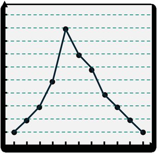
• Frequency Polygon: Connects points representing frequencies at class midpoints with line segments.

• Stemplot (Stem-and-Leaf Plot): Displays actual data values, showing both the distribution and the individual values.

Frequency Distributions

Constructing Frequency Distributions

A frequency distribution is a table that shows the frequency of data values within specified intervals (classes). It helps summarize large datasets and identify patterns.

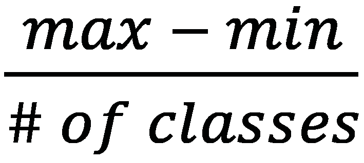
• Class Width: The difference between consecutive lower (or upper) class limits. Calculated as:

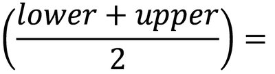
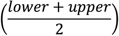
• Class Midpoint: The average of the lower and upper class limits.

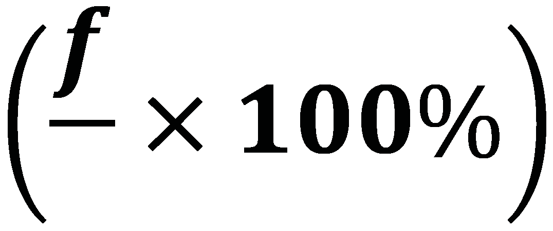
• Relative Frequency: The proportion of data values in each class, often expressed as a percentage.

Steps to Create a Frequency Distribution

1. Calculate class width and round up to a convenient number.

2. Determine lower class limits, starting at or below the minimum data value.

3. Determine upper class limits, typically as one less than the next lower class limit.

4. Tally each data value into its appropriate class.

Histograms

Understanding Histograms

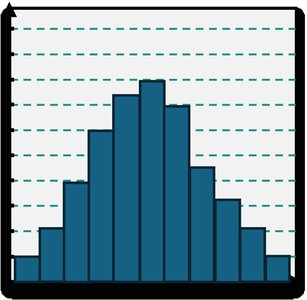
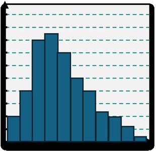
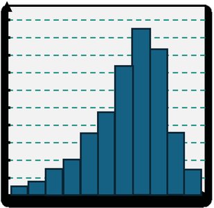
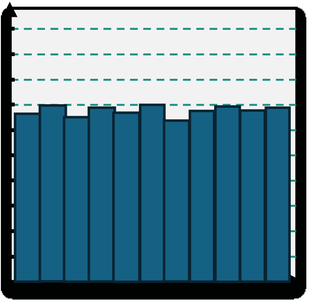
Histograms are graphical representations of frequency distributions for quantitative data. They use vertical bars to show the frequency of data within each class interval.

• Horizontal Axis: Represents class intervals or midpoints.

• Vertical Axis: Represents frequency.

• Distribution Shapes: Common shapes include normal (bell-shaped), skewed right, skewed left, and uniform.

Bar Graphs & Pareto Charts

Bar Graphs

Bar graphs are used to display categorical data. The height or length of each bar represents the frequency or count for each category.

• Pareto Chart: A special bar graph where categories are ordered from highest to lowest frequency.

Pie Charts

Pie Charts

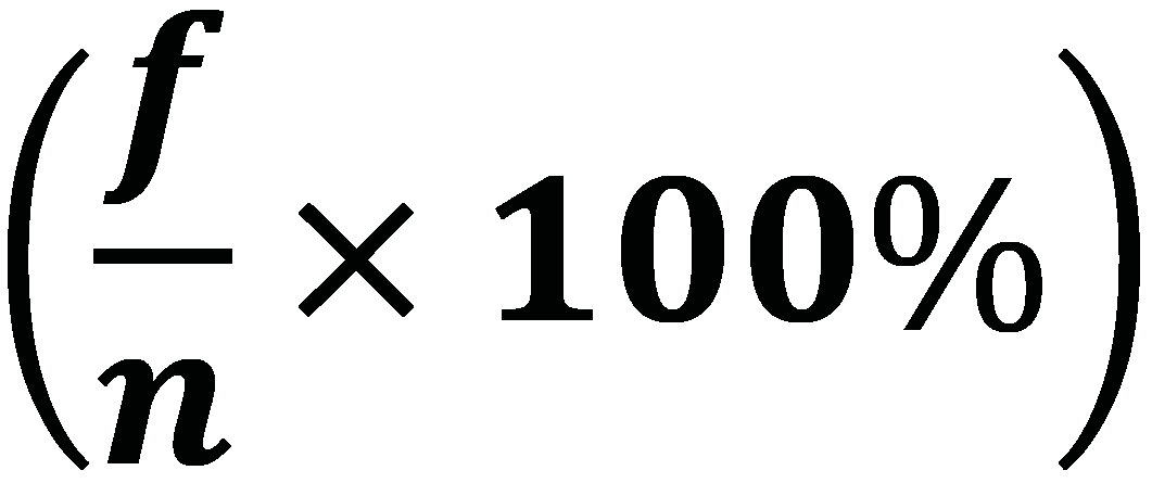
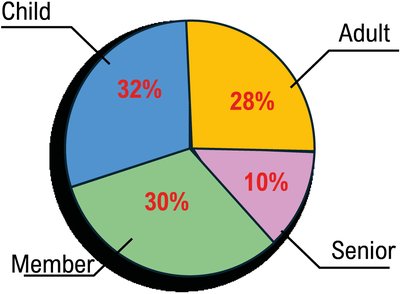
Pie charts visually represent the proportion of each category in a dataset. Each slice corresponds to a category, and its size is proportional to the percentage of responses.

• Percentage Calculation:

Frequency Polygons

Frequency Polygons

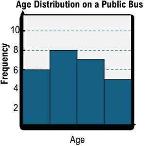
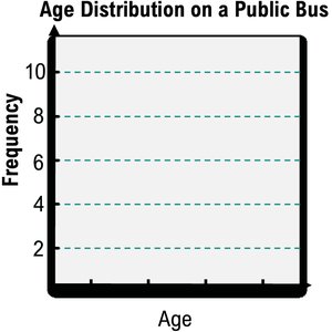
Frequency polygons are line graphs that connect points representing the frequency at each class midpoint. They are useful for comparing distributions and visualizing trends.

• Class Midpoint Formula:

Dotplots

Dotplots

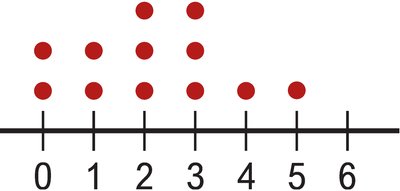
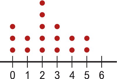
Dotplots are simple graphs for displaying quantitative data. Each dot represents a data point, and dots are stacked above a number line for each value.

Stemplots (Stem-and-Leaf Plots)

Stemplots

Stemplots display quantitative data by splitting each value into a "stem" (all but the rightmost digit) and a "leaf" (the rightmost digit). This allows for quick visualization of the distribution and retention of actual data values.

• How to Create:

  1. Order data from smallest to largest.

  2. Draw a vertical line to separate stems and leaves.

  3. List stems in the left column and leaves in the right column.

Time-Series Graphs

Time-Series Graphs

Time-series graphs plot data points over time, connecting them with line segments to show trends. The x-axis represents time, and the y-axis represents the measured value.

Summary Table: Types of Graphs and Their Uses

Additional info: These notes expand on brief points from the original material, providing definitions, formulas, and examples for each graph type. All included images directly illustrate the graph types and formulas discussed in the adjacent paragraphs.