Probability and Probability Distributions

Basic Definitions of Probability

Probability theory is fundamental in statistics and decision-making, especially in business and finance. It quantifies uncertainty and helps managers make informed decisions under risk. Probability is used to analyze sales trends, customer behavior, inventory levels, and more.

• Probability: A numerical measure (between 0 and 1) of the likelihood that an event will occur.

• Experiment: Any process of observation or measurement that generates well-defined outcomes (e.g., tossing a coin, rolling a die).

• Sample Space (S): The set of all possible outcomes of an experiment.

• Event: A subset of the sample space; a statement about one or more outcomes.

• Outcome: The result of a single trial of an experiment.

Example: Rolling a die: S = {1,2,3,4,5,6}. Event A (odd numbers) = {1,3,5}.

Key Probability Concepts

• Equally Likely Events: Events with the same chance of occurring.

• Mutually Exclusive Events: Events that cannot occur simultaneously.

• Complement of an Event (A'): All outcomes in the sample space not in event A.

• Elementary Event: An event with only one outcome.

• Compound Event: An event with more than one outcome.

• Intersection (A ∩ B): Outcomes common to both events A and B.

• Union (A ∪ B): Outcomes in A, B, or both.

• Independent Events: The occurrence of one does not affect the probability of the other.

• Dependent Events: The occurrence of one affects the probability of the other.

Approaches to Measuring Probability

• Classical Approach: Used when all outcomes are equally likely. , where n(A) is the number of favorable outcomes and N is the total number of outcomes.

• Relative Frequency Approach: Probability is the long-run proportion of times an event occurs in repeated trials.

• Axiomatic Approach: Probability is defined by axioms:

  • If A and B are mutually exclusive:

  • General addition rule:

• Subjective Approach: Probability is based on personal judgment or prior knowledge.

Conditional Probability and Independence

Conditional probability measures the likelihood of event A given that event B has occurred:

• , provided

• For independent events:

Example: If , , , then A and B are independent because .

Random Variables and Probability Distributions

Random Variables

A random variable assigns a real number to each outcome in the sample space. There are two types:

• Discrete Random Variable: Takes countable values (e.g., number of customers).

• Continuous Random Variable: Takes any value within an interval (e.g., time, height).

Probability Distributions

• Discrete Probability Distribution: Lists all possible values of a discrete random variable and their probabilities.

• Continuous Probability Distribution: Described by a probability density function (pdf) , where:

  • for all x

Expectation and Variance

• Expected Value (Mean):

  • Discrete:

  • Continuous:

• Variance:

  • Discrete:

  • Continuous:

Common Discrete Probability Distributions

Binomial Distribution

The binomial distribution models the number of successes in n independent trials, each with probability p of success.

• Probability mass function: , for

• Mean:

• Variance:

Example: Probability of 3 successes in 10 trials with :

Poisson Distribution

The Poisson distribution models the number of events in a fixed interval of time or space, given the average rate λ.

• Probability mass function: , for

• Mean and Variance:

Example: Probability of 1 customer arriving in a minute when λ = 4:

Common Continuous Probability Distributions

Normal Distribution

The normal distribution is a continuous, symmetric, bell-shaped distribution defined by its mean (μ) and standard deviation (σ):

• Probability density function:

• Total area under the curve is 1.

• Mean = Median = Mode = μ

• Standardization: , where Z follows the standard normal distribution

Probabilities are found using the area under the curve between two points, often with the help of Z-tables.

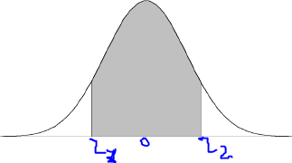
Example: Probability that Z is between z1 and z2 is the shaded area under the curve between those points.

Properties of the Standard Normal Distribution

• Mean = 0, Standard deviation = 1

• Symmetrical about the mean

• Area to the left of Z = 0 is 0.5

• Probabilities for any interval can be found using standard normal tables

Applications of the Normal Distribution

• Finding probabilities for intervals (e.g., )

• Calculating probabilities for real-world scenarios (e.g., investment returns, heights, test scores)

• Standardizing values to compare different normal distributions

Example: If returns are normally distributed with mean 10% and standard deviation 5%, the probability of a negative return is .