
Ch. 10 - Chi-Square Tests and the F-Distribution
Larson - Elementary Statistics: Picturing the World 8th Edition
Larson8th EditionElementary Statistics: Picturing the WorldISBN: 9780137493470당신이 사용하는 게 아니라요?교과서 변경
10장, 문제 10.1.10b

Performing a Chi-Square Goodness-of-Fit Test
In Exercises 7–16, (b) find the critical value and identify the rejection region.


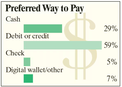
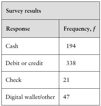
Ways to Pay A financial analyst claims that the distribution of people’s preferences on how to pay for goods is different from the distribution shown in the figure. You randomly select 600 people and record their preferences on how to pay for goods. The table shows the results. At α=0.01, test the financial analyst’s claim. (Adapted from Travis Credit Union)


검증된 단계별 안내
1
Step 1: State the null hypothesis (H₀) and the alternative hypothesis (H₁). The null hypothesis assumes that the observed distribution matches the expected distribution shown in the figure. The alternative hypothesis claims that the observed distribution is different from the expected distribution.
Step 2: Calculate the expected frequencies for each category based on the percentages provided in the figure and the total sample size of 600 people. Use the formula: Expected frequency = (Percentage / 100) × Total sample size. For example, for 'Cash', the expected frequency is (29 / 100) × 600.
Step 3: Compute the Chi-Square test statistic using the formula: χ² = Σ((Observed frequency - Expected frequency)² / Expected frequency). Perform this calculation for each category (Cash, Debit or credit, Check, Digital wallet/other) and sum the results.
Step 4: Determine the critical value for the Chi-Square test at α = 0.01 and degrees of freedom (df). The degrees of freedom are calculated as df = (Number of categories - 1). Use a Chi-Square distribution table to find the critical value.
Step 5: Compare the calculated Chi-Square test statistic to the critical value. If the test statistic exceeds the critical value, reject the null hypothesis (H₀). Otherwise, fail to reject the null hypothesis. Interpret the result in the context of the financial analyst's claim.

비슷한 문제에 대한 검증된 영상 답변:

이 영상 해법은 위 문제에 도움이 된다고 튜터들이 추천한 것입니다.
영상 길이:
2m

주요 개념

질문에 올바르게 답하기 위해 반드시 이해해야 하는 핵심 개념들은 다음과 같습니다.

Chi-Square Goodness-of-Fit Test

The Chi-Square Goodness-of-Fit Test is a statistical method used to determine if the observed frequencies of a categorical variable differ significantly from the expected frequencies based on a specific hypothesis. It compares the actual data collected from a sample to a theoretical distribution, allowing researchers to assess whether the sample data fits the expected distribution.
추천 영상:
가이드 코스
10:17
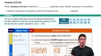
Goodness of Fit Test

Critical Value

The critical value in hypothesis testing is a threshold that determines the boundary for rejecting the null hypothesis. It is derived from the chosen significance level (α), which indicates the probability of making a Type I error. In this case, with α=0.01, the critical value will help identify the rejection region for the Chi-Square statistic, indicating where the observed data would be considered significantly different from the expected distribution.
추천 영상:
가이드 코스
05:50
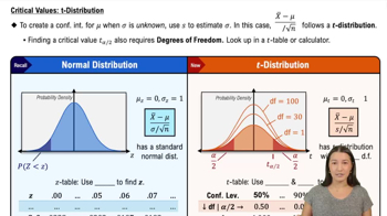
Critical Values: t-Distribution

Rejection Region

The rejection region is the range of values for the test statistic that leads to the rejection of the null hypothesis. In the context of the Chi-Square Goodness-of-Fit Test, if the calculated Chi-Square statistic falls within this region, it suggests that the observed distribution of preferences significantly differs from the expected distribution, supporting the financial analyst's claim.
추천 영상:
가이드 코스
09:56
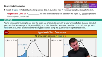
Step 4: State Conclusion
관련 실천
교과서 질문

Performing a Chi-Square Goodness-of-Fit Test

In Exercises 7–16, (a) identify the claim and state H₀ and Hₐ.


Ways to Pay A financial analyst claims that the distribution of people’s preferences on how to pay for goods is different from the distribution shown in the figure. You randomly select 600 people and record their preferences on how to pay for goods. The table shows the results. At α=0.01, test the financial analyst’s claim. (Adapted from Travis Credit Union)


71
views
교과서 질문

In each exercise,

e. interpret the decision in the context of the original claim.

[APPLET] In Exercises 1–3, use the data, which list the hourly wages (in dollars) for randomly selected surgical technologists from three states. Assume the wages are normally distributed and that the samples are independent. (Adapted from U.S. Bureau of Labor Statistics)

Maine: 22.76, 27.60, 25.08, 17.01, 30.15, 27.09, 20.95, 25.52, 20.11, 23.67, 24.32

Oklahoma: 24.64, 21.66, 19.38, 18.19, 23.14, 20.58, 19.53, 30.77, 27.46, 23.80

Massachusetts: 27.07, 24.71, 32.80, 28.34, 33.45, 33.36, 36.81, 30.04, 29.01, 24.30, 29.22, 29.50

Are the mean hourly wages of surgical technologists the same for all three states? Use α=0.01. Assume that the population variances are equal.

21
views
교과서 질문

Performing a Chi-Square Goodness-of-Fit Test

In Exercises 7–16, (c) find the chi-square test statistic.


Ways to Pay A financial analyst claims that the distribution of people’s preferences on how to pay for goods is different from the distribution shown in the figure. You randomly select 600 people and record their preferences on how to pay for goods. The table shows the results. At α=0.01, test the financial analyst’s claim. (Adapted from Travis Credit Union)


67
views
교과서 질문

Performing a Chi-Square Goodness-of-Fit Test

In Exercises 7–16, (d) decide whether to reject or fail to reject the null hypothesis.


Ways to Pay A financial analyst claims that the distribution of people’s preferences on how to pay for goods is different from the distribution shown in the figure. You randomly select 600 people and record their preferences on how to pay for goods. The table shows the results. At α=0.01, test the financial analyst’s claim. (Adapted from Travis Credit Union)


79
views
교과서 질문

In each exercise,

d. decide whether to reject or fail to reject the null hypothesis, and

[APPLET] In Exercises 1–3, use the data, which list the hourly wages (in dollars) for randomly selected surgical technologists from three states. Assume the wages are normally distributed and that the samples are independent. (Adapted from U.S. Bureau of Labor Statistics)

Maine: 22.76, 27.60, 25.08, 17.01, 30.15, 27.09, 20.95, 25.52, 20.11, 23.67, 24.32

Oklahoma: 24.64, 21.66, 19.38, 18.19, 23.14, 20.58, 19.53, 30.77, 27.46, 23.80

Massachusetts: 27.07, 24.71, 32.80, 28.34, 33.45, 33.36, 36.81, 30.04, 29.01, 24.30, 29.22, 29.50

Are the mean hourly wages of surgical technologists the same for all three states? Use α=0.01. Assume that the population variances are equal.

21
views
교과서 질문

List the two conditions that must be met in order to use the paired-sample sign test.

100
views