Ch. 2 - Descriptive Statistics
Larson - Elementary Statistics: Picturing the World 8th Edition
Larson8th EditionElementary Statistics: Picturing the WorldISBN: 9780137493470당신이 사용하는 게 아니라요?교과서 변경
2장, 문제 2.4.45

Comparing Variation in Different Data Sets In Exercises 45–50, find the coefficient of variation for each of the two data sets. Then compare the results.
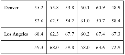
Annual Salaries Sample annual salaries (in thousands of dollars) for entry level architects in Denver, CO, and Los Angeles, CA, are listed.
Table comparing annual salaries (in thousands) for entry-level architects in Denver and Los Angeles.

검증된 단계별 안내
1
Step 1: Understand the coefficient of variation (CV). The CV is a measure of relative variability and is calculated as the ratio of the standard deviation (SD) to the mean (μ), expressed as a percentage: CV = (SD / μ) × 100.
Step 2: Calculate the mean (μ) for each data set. Add all the values in the Denver data set and divide by the number of values to find the mean for Denver. Repeat the process for the Los Angeles data set.
Step 3: Calculate the standard deviation (SD) for each data set. Use the formula for SD: SD = sqrt(Σ(xᵢ - μ)² / (n - 1)), where xᵢ represents each data point, μ is the mean, and n is the number of data points. Perform this calculation for both Denver and Los Angeles data sets.
Step 4: Compute the coefficient of variation (CV) for each data set using the formula CV = (SD / μ) × 100. Substitute the mean and standard deviation values calculated in the previous steps for both Denver and Los Angeles.
Step 5: Compare the CVs of the two data sets. The data set with the higher CV has greater relative variability in annual salaries.

비슷한 문제에 대한 검증된 영상 답변:

이 영상 해법은 위 문제에 도움이 된다고 튜터들이 추천한 것입니다.
영상 길이:
9m
도움이 되었나요?

주요 개념

질문에 올바르게 답하기 위해 반드시 이해해야 하는 핵심 개념들은 다음과 같습니다.

Coefficient of Variation

The coefficient of variation (CV) is a statistical measure of the relative variability of a data set. It is calculated as the ratio of the standard deviation to the mean, expressed as a percentage. A higher CV indicates greater dispersion relative to the mean, making it useful for comparing the degree of variation between different data sets, especially when the means are significantly different.
추천 영상:
가이드 코스
06:14
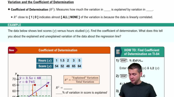
Coefficient of Determination

Standard Deviation

Standard deviation is a measure of the amount of variation or dispersion in a set of values. It quantifies how much the individual data points deviate from the mean of the data set. A low standard deviation indicates that the data points tend to be close to the mean, while a high standard deviation indicates that the data points are spread out over a wider range of values.
추천 영상:
가이드 코스
08:45
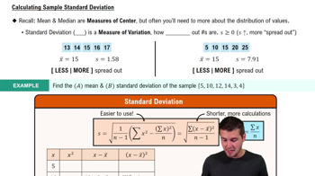
Calculating Standard Deviation

Mean

The mean, or average, is a measure of central tendency that is calculated by summing all the values in a data set and dividing by the number of values. It provides a single value that represents the center of the data distribution. The mean is sensitive to extreme values (outliers), which can skew the results, making it important to consider alongside other measures of central tendency and variability.
추천 영상:
가이드 코스
04:52
Calculating the Mean
관련 실천
교과서 질문

Finding the Mean of a Frequency Distribution In Exercises 49–52, approximate the mean of the frequency distribution.


Social Media The average daily amounts of time (in minutes) spent on Snapchat

267
views
교과서 질문

Finding z-Scores The distribution of the ages of the winners of the Tour de France from 1903 to 2020 is approximately bell-shaped. The mean age is 27.9 years, with a standard deviation of 3.4 years. In Exercises 43–48, use the corresponding z-score to determine whether the age is unusual. Explain your reasoning. (Source: Le Tour de France)


100
views
교과서 질문

Finding a Weighted Mean In Exercises 41– 46, find the weighted mean of the data.


Grades A student receives the grades shown below, with an A worth 4 points, a B worth 3 points, a C worth 2 points, and a D worth 1 point. What is the student’s grade point average?


238
views
교과서 질문

Finding the Mean of a Frequency Distribution In Exercises 49–52, approximate the mean of the frequency distribution.


Populations The populations (in thousands) of the counties in Montana in 2019 (Source: U.S. Census Bureau)

126
views
교과서 질문

Constructing a Frequency Distribution and a Frequency Polygon In Exercises 35 and 36, construct a frequency distribution and a frequency polygon for the data set using the indicated number of classes. Describe any patterns.

Declaration of Independence

Number of classes: 5

Data set: Number of children of those who signed the Declaration of Independence (Source: The U.S. National Archives & Records Administration) 5 2 12 18 7 4 10 8 16 3 3 7 3 1 2 7 13 0 8 3 7 5 2 6 0 6 7 9 0 11 9 10 7 8 13 5 8 3 5 0 3 13 3 15 5 6 3 2 5 2 0 3 7 12 4 1

95
views
교과서 질문

Graphical Analysis In Exercises 19–22, use the box-and-whisker plot to determine whether the shape of the distribution represented is symmetric, skewed left, skewed right, or none of these. Justify your answer.

100
views