Ch. 10 - Correlation and Regression
Triola - Elementary Statistics 14th Edition
Triola14th EditionElementary StatisticsISBN: 9780137366446당신이 사용하는 게 아니라요?교과서 변경
10장, 문제 10.3.17a

Variation and Prediction Intervals
In Exercises 17–20, find the (a) explained variation, (b) unexplained variation, and (c) indicated prediction interval. In each case, there is sufficient evidence to support a claim of a linear correlation, so it is reasonable to use the regression equation when making predictions.
Altitude and Temperature Listed below are altitudes (thousands of feet) and outside air temperatures (°F) recorded by the author during Delta Flight 1053 from New Orleans to Atlanta. For the prediction interval, use a 95% confidence level with the altitude of 6327 ft (or 6.327 thousand feet).
Table showing altitudes (3 to 33k feet) and corresponding temperatures (57°F to -54°F) from a flight.

검증된 단계별 안내
1
Step 1: Begin by calculating the regression equation (y = mx + b) using the given data. To do this, compute the slope (m) and y-intercept (b) using the formulas: m = (Σ(xy) - n(μx)(μy)) / (Σ(x^2) - n(μx^2)) and b = μy - mμx, where μx and μy are the means of x (altitude) and y (temperature).
Step 2: Compute the explained variation (SS_reg). This is the sum of squared differences between the predicted values (ŷ) and the mean of the observed values (μy). Use the formula: SS_reg = Σ(ŷ - μy)^2.
Step 3: Compute the unexplained variation (SS_res). This is the sum of squared differences between the observed values (y) and the predicted values (ŷ). Use the formula: SS_res = Σ(y - ŷ)^2.
Step 4: Calculate the total variation (SS_tot) as the sum of explained and unexplained variations: SS_tot = SS_reg + SS_res. Verify that this relationship holds true.
Step 5: For the prediction interval at an altitude of 6327 ft (6.327 thousand feet), use the regression equation to predict the temperature (ŷ). Then, calculate the margin of error using the standard error of the estimate and the t-value for a 95% confidence level. The prediction interval is given by: ŷ ± margin of error.

비슷한 문제에 대한 검증된 영상 답변:

이 영상 해법은 위 문제에 도움이 된다고 튜터들이 추천한 것입니다.
영상 길이:
11m
도움이 되었나요?

주요 개념

질문에 올바르게 답하기 위해 반드시 이해해야 하는 핵심 개념들은 다음과 같습니다.

Explained Variation

Explained variation refers to the portion of the total variation in the dependent variable (in this case, temperature) that can be attributed to the independent variable (altitude). It is calculated using the regression model, where the sum of squares of the regression (SSR) indicates how much of the variation is explained by the model. A higher explained variation suggests a stronger relationship between the variables.
추천 영상:
가이드 코스
06:14
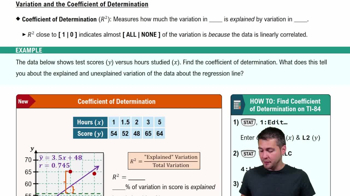
Coefficient of Determination

Unexplained Variation

Unexplained variation, also known as residual variation, is the part of the total variation in the dependent variable that cannot be accounted for by the independent variable. It is represented by the sum of squares of the residuals (SSE) in a regression analysis. Understanding unexplained variation is crucial for assessing the accuracy of predictions made by the regression model, as it indicates the degree of error in the predictions.
추천 영상:
가이드 코스
06:14
Coefficient of Determination

Prediction Interval

A prediction interval provides a range of values within which we expect a future observation to fall, given a certain level of confidence (e.g., 95%). It takes into account both the variability of the data and the uncertainty in the regression model. The prediction interval is wider than the confidence interval for the mean response because it includes the additional variability of individual observations, making it essential for making informed predictions.
추천 영상:
가이드 코스
09:00
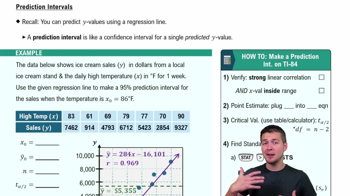
Prediction Intervals
관련 실천
교과서 질문

Effects of Clusters Refer to the Minitab-generated scatterplot given in Exercise 10 of Section 10-1.


a. Using the pairs of values for all 8 points, find the equation of the regression line.

173
views
교과서 질문

Explore!

Exercises 11 and 12 provide two data sets from “Graphs in Statistical Analysis,” by F. J. Anscombe, the American Statistician, Vol. 27. For each exercise,


a. Construct a scatterplot.

155
views
교과서 질문

Least-Squares Property According to the least-squares property, the regression line minimizes the sum of the squares of the residuals. Refer to the jackpot/tickets data in Table 10-1 and use the regression equation y^ = -10.9 + 0.174x that was found in Examples 1 and 2 of this section.

b. Find the sum of the squares of the residuals.

302
views
교과서 질문

Clusters Refer to the Minitab-generated scatterplot. The four points in the lower left corner are measurements from women, and the four points in the upper right corner are from men.

a. Examine the pattern of the four points in the lower left corner (from women) only, and subjectively determine whether there appears to be a correlation between x and y for women.

146
views
교과서 질문

Outlier Refer to the accompanying Minitab-generated scatterplot.

b. After identifying the 10 pairs of coordinates corresponding to the 10 points, find the value of the correlation coefficient r and determine whether there is a linear correlation.

134
views
교과서 질문

Notation The author conducted an experiment in which the height of each student was measured in centimeters and those heights were matched with the same students’ scores on the first statistics test.

b. Without doing any research or calculations, estimate the value of r.

249
views