Ch. 2 - Exploring Data with Tables and Graphs
Triola - Elementary Statistics 14th Edition
Triola14th EditionElementary StatisticsISBN: 9780137366446당신이 사용하는 게 아니라요?교과서 변경
2장, 문제 2.4.4d

Estimating r For each of the following, estimate the value of the linear correlation coefficient r for the given paired data obtained from 50 randomly selected adults.


d. The 50 adults all drove cars from Jacksonville, Florida, to Richmond, Virginia. Their average (mean) speeds are recorded along with the times it took to complete that trip.

검증된 단계별 안내
1
Understand the problem: The goal is to estimate the linear correlation coefficient (r), which measures the strength and direction of the linear relationship between two variables. Here, the variables are the average speeds of the cars and the times it took to complete the trip.
Recall the properties of the correlation coefficient (r): It ranges from -1 to 1. A value close to -1 indicates a strong negative linear relationship, a value close to 1 indicates a strong positive linear relationship, and a value near 0 indicates no linear relationship.
Analyze the relationship between the variables: As the average speed increases, the time taken to complete the trip is expected to decrease. This suggests a negative linear relationship between speed and time.
Visualize the data: If possible, create a scatterplot of the data points with average speed on the x-axis and time on the y-axis. Look for a downward trend in the points, which would confirm a negative correlation.
Estimate the value of r: Based on the observed trend in the scatterplot or the relationship described, estimate r as a negative value closer to -1 if the points form a strong linear pattern, or closer to 0 if the pattern is weak or scattered.

비슷한 문제에 대한 검증된 영상 답변:

이 영상 해법은 위 문제에 도움이 된다고 튜터들이 추천한 것입니다.
영상 길이:
2m
도움이 되었나요?

주요 개념

질문에 올바르게 답하기 위해 반드시 이해해야 하는 핵심 개념들은 다음과 같습니다.

Linear Correlation Coefficient (r)

The linear correlation coefficient, denoted as r, quantifies the strength and direction of a linear relationship between two variables. Its value ranges from -1 to 1, where 1 indicates a perfect positive correlation, -1 indicates a perfect negative correlation, and 0 indicates no correlation. Understanding r is crucial for interpreting how changes in one variable may relate to changes in another.
추천 영상:
가이드 코스
05:43
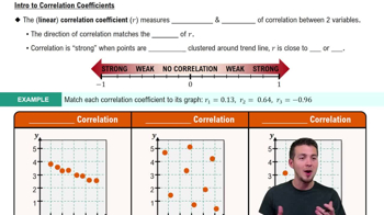
Correlation Coefficient

Mean Speed and Time Relationship

In the context of the given data, the mean speed of the cars and the time taken for the trip are two variables that can be analyzed for correlation. Typically, as speed increases, the time taken to complete a trip decreases, suggesting a negative correlation. Analyzing this relationship helps in understanding how these two factors interact in real-world scenarios.
추천 영상:
04:36
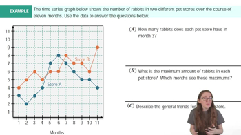
Time-Series Graphs Example 1

Random Sampling

Random sampling is a technique used to select a subset of individuals from a larger population, ensuring that every individual has an equal chance of being chosen. This method is essential for obtaining unbiased data, which enhances the validity of statistical analyses. In this case, the 50 randomly selected adults provide a representative sample for estimating the correlation between speed and time.
추천 영상:
05:11
Sampling Distribution of Sample Proportion
관련 실천
교과서 질문

Interpreting Normal Quantile Plots Which of the following normal quantile plots appear to represent data from a population having a normal distribution? Explain.

204
views

교과서 질문

In Exercises 1–5, use the data listed in the margin, which are magnitudes (Richter scale) and depths (km) of earthquakes from Data Set 24 “Earthquakes” in Appendix B

[Image]

Frequency Distribution For the frequency distribution from Exercise 1, find the following.


a. Class limits of the first class

b. Class boundaries of the first class

c. Class midpoint of the first class

162
views
교과서 질문

In Exercises 1–5, use the data listed in the margin, which are magnitudes (Richter scale) and depths (km) of earthquakes from Data Set 24 “Earthquakes” in Appendix B

Frequency Distribution Construct a frequency distribution of the magnitudes. Use a class width of 0.50 and use a starting value of 1.00.

107
views
교과서 질문

In Exercises 1–5, use the data listed in the margin, which are magnitudes (Richter scale) and depths (km) of earthquakes from Data Set 24 “Earthquakes” in Appendix B


Histogram Construct the histogram corresponding to the frequency distribution from Exercise 1. For the values on the horizontal axis, use the class midpoint values. Which of the following comes closest to describing the distribution: uniform, normal, skewed left, skewed right?


113
views
교과서 질문

Tornado Alley Using the same frequency distribution from Exercise 1, identify the class limits of the first class and the class boundaries of the first class.

142
views
교과서 질문

Tornado Alley Construct the relative frequency distribution corresponding to the frequency distribution in Exercise 1

146
views