Chapter 6: Demand and Supply Elasticity – Microeconomics Study Notes

Chapter 6: Demand and Supply Elasticity

Introduction

This chapter explores how demand and supply respond to changes in price and income, and the implications for firm revenues. Understanding elasticity is crucial for making informed pricing and production decisions in microeconomics.

Price Elasticity of Demand

Definition and Concept

Price elasticity of demand measures how sensitive the quantity demanded of a good is to changes in its price. It is always negative due to the law of demand, which states that price and quantity demanded move in opposite directions.

• Formula: $E_p = \frac{\%\ \text{change in quantity demanded}}{\%\ \text{change in price}}$

• Relative Quantities: Elasticity uses percentage changes, making it independent of units (e.g., grams, dollars).

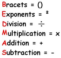
• Order of Operations: When calculating, follow BEDMAS (Brackets, Exponents, Division, Multiplication, Addition, Subtraction).

Examples of Price Sensitivity

Consumers may respond differently to price changes depending on the product:

• Toothpaste: Often inelastic due to necessity and few substitutes.

• Cell phones: More elastic, as alternatives exist and price is significant.

• Gasoline: Typically inelastic in the short run, but more elastic in the long run.

Calculating Price Elasticity of Demand

Use the midpoint (average) formula for accuracy:

• $E_p = \frac{(Q_2 - Q_1) / ((Q_2 + Q_1)/2)}{(P_2 - P_1) / ((P_2 + P_1)/2)}$

• Ignore the negative sign for practical purposes.

International Policy Example: Tesla Vehicles in Hong Kong

When subsidies were removed, Tesla prices rose from $75,000 to $130,000, and monthly demand dropped from 500 to 30. The price elasticity of demand was calculated as 3.3, indicating highly elastic demand.

Interpretation: A 1% increase in price led to a 3.3% decrease in quantity demanded.

Ranges of Price Elasticity

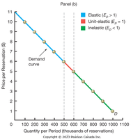
• Elastic Demand (Ep > 1): Quantity demanded is highly responsive to price changes (e.g., steak dinner).

• Unit Elasticity (Ep = 1): Quantity demanded changes proportionally to price.

• Inelastic Demand (Ep < 1): Quantity demanded is less responsive (e.g., electricity, insulin).

Extreme Cases

• Perfectly Inelastic Demand (Ep = 0): Quantity demanded does not change with price (vertical demand curve).

• Perfectly Elastic Demand (Ep = ∞): Any price increase drops quantity demanded to zero (horizontal demand curve).

Elasticity and Total Revenues

Relationship Between Elasticity and Revenue

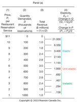
Total Revenue (TR) is the product of price and quantity: $TR = P \times Q$. The effect of price changes on TR depends on elasticity:

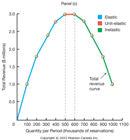
• Elastic Demand: Price and TR move in opposite directions.

• Unit Elastic Demand: TR remains unchanged when price changes.

• Inelastic Demand: Price and TR move in the same direction.

Example: If cell phone price increases by 5% and quantity demanded decreases by 10%, TR decreases (elastic demand).

Graphical Representation

Tables and graphs illustrate how elasticity affects total revenue for restaurant reservations:

Determinants of Price Elasticity of Demand

Key Determinants

• Existence of Substitutes: More substitutes make demand more elastic (e.g., Maple Leaf Bacon vs. generic bacon).

• Share of Budget: Goods that take up a larger share of budget are more elastic (e.g., European vacation vs. salt).

• Time for Adjustment: Demand is more elastic in the long run as consumers adjust their behavior.

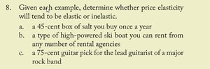
Example: Demand for salt is inelastic due to low budget share and few substitutes; demand for rental ski boats is elastic due to many substitutes and higher cost.

Short-Run vs. Long-Run Elasticity

Elasticity increases over time as consumers find alternatives and adjust consumption patterns. In the short run, demand for necessities (e.g., gasoline) is inelastic, but becomes more elastic in the long run.

Cross Price Elasticity and Income Elasticity of Demand

Cross Price Elasticity (Exy)

Measures the responsiveness of demand for one good to changes in the price of another good:

• $E_{xy} = \frac{\%\ \text{change in quantity demanded of Good X}}{\%\ \text{change in price of Good Y}}$

• Positive Exy: Goods are substitutes.

• Negative Exy: Goods are complements.

Income Elasticity of Demand (Ei)

Measures how demand changes with consumer income:

• $E_i = \frac{\%\ \text{change in quantity demanded}}{\%\ \text{change in income}}$

• Positive Ei: Normal goods.

• Negative Ei: Inferior goods.

Price is assumed constant when calculating income elasticity.

Price Elasticity of Supply

Definition and Extremes

Price elasticity of supply measures how responsive quantity supplied is to price changes:

• Perfectly Elastic Supply: Any price decrease drops quantity supplied to zero (horizontal supply curve).

• Perfectly Inelastic Supply: Quantity supplied remains constant regardless of price (vertical supply curve).

Determinants of Supply Elasticity

• Time for Adjustment: Longer adjustment periods increase elasticity.

• Availability of Raw Materials: Limited materials make supply inelastic.

• Complexity of Production: More complex production processes reduce elasticity.

• Excess Capacity and Inventories: Excess capacity increases elasticity.

As time passes, supply becomes more elastic as firms can adjust production and new firms can enter the market.

Summary of Learning Objectives

• Calculate price elasticity of demand using percentage changes.

• Understand the relationship between elasticity and total revenue.

• Identify determinants of price elasticity of demand: substitutes, budget share, time for adjustment.

• Explain cross price and income elasticities of demand.

• Classify supply elasticities and understand how adjustment time affects supply elasticity.