Chapter 6: Firms and Production – Microeconomics Study Notes

Firms and Production

Ownership and Management of Firms

Firms are organizations that transform inputs into outputs, producing goods and services for sale. The structure and management of firms vary depending on their ownership and objectives.

• Firm: An entity that converts labor, materials, energy, and capital into outputs.

• Types of Firms:

  • Private sector: Owned by individuals or nongovernmental entities, aiming for profit.

  • Public sector: Owned by government agencies.

  • Nonprofit sector: Not government-owned and not intended to earn profit.

• Ownership Structures:

  • Sole proprietorship: Owned and run by one individual.

  • General partnership: Jointly owned and controlled by two or more people.

  • Corporation: Owned by shareholders; owners have limited liability.

Profit Maximization and Efficiency

Owners of firms are assumed to maximize profit, which is the difference between revenues and costs. Efficient production is achieved when a firm cannot produce the current output with fewer inputs, given existing technology.

• Profit formula: $\pi = R - C$

• Technological efficiency: Producing output with the minimum required inputs.

Inputs and Production Process

Firms use various inputs to produce outputs. The main categories of inputs are capital, labor, and materials.

• Capital (K): Long-lived inputs such as land, buildings, and equipment.

• Labor (L): Human services, including managers, skilled, and less-skilled workers.

• Materials (M): Raw goods and processed products.

Production Function

The production function describes the relationship between input quantities and the maximum output achievable, given current technology.

• General form: $q = f(L, K)$

• Inputs: Labor (L) and Capital (K)

• Output: Quantity produced (q)

Time and Variability of Inputs

Inputs can be classified as fixed or variable depending on the time frame considered.

• Short run: At least one input is fixed.

• Long run: All inputs are variable.

• Fixed input: Cannot be varied in the short run.

• Variable input: Can be changed readily.

Short-Run Production

In the short run, the production function is typically expressed as $q = f(L, K)$, where capital (K) is fixed and labor (L) is variable.

Total, Marginal, and Average Product of Labor

These concepts measure the productivity of labor in the short run.

• Total Product of Labor (TPL): Total output produced by a given amount of labor.

• Marginal Product of Labor (MPL): Change in output from an additional unit of labor. $MPL = \frac{\Delta q}{\Delta L}$

• Average Product of Labor (APL): Output per worker. $APL = \frac{q}{L}$

Law of Diminishing Marginal Returns

If a firm increases one input while holding others constant, the additional output from each extra unit of input will eventually decrease.

• Diminishing marginal returns: Marginal product of an input decreases as more of it is used.

Long-Run Production and Isoquants

In the long run, both labor and capital are variable, and firms can substitute between them to maintain output. Isoquants represent combinations of inputs that yield the same output.

• Isoquant: Curve showing efficient combinations of labor and capital for a given output. $q = f(L, K)$

• Properties of Isoquants:

  • Further from origin = higher output

  • Do not cross

  • Downward sloping

Substitutability of Inputs and Marginal Rate of Technical Substitution (MRTS)

The MRTS measures how many units of one input are needed to replace one unit of another input while keeping output constant. It is the slope of the isoquant.

• MRTS formula: $MRTS = \frac{\Delta K}{\Delta L}$

• Along an isoquant: $(MPL \times \Delta L) + (MPK \times \Delta K) = 0$

Returns to Scale

Returns to scale describe how output changes when all inputs are increased proportionately.

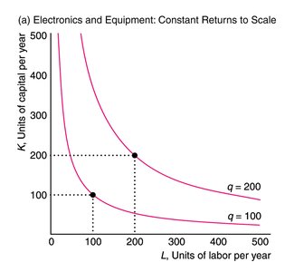
• Constant Returns to Scale (CRS): Output increases by the same percentage as inputs. $f(2L, 2K) = 2f(L, K)$

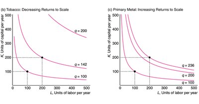
• Increasing Returns to Scale (IRS): Output increases by more than the percentage increase in inputs. $f(2L, 2K) > 2f(L, K)$

• Decreasing Returns to Scale (DRS): Output increases by less than the percentage increase in inputs. $f(2L, 2K) < 2f(L, K)$

Cobb-Douglas Production Function

The Cobb-Douglas function is widely used to model production. The sum of the exponents determines returns to scale.

• Formula: $q = AL^{\alpha}K^{\beta}$

• Returns to scale: $\gamma = \alpha + \beta$

  • $\gamma = 1$ : Constant returns to scale

  • $\gamma > 1$ : Increasing returns to scale

  • $\gamma < 1$ : Decreasing returns to scale

Productivity and Technical Change

Productivity differences arise from technological or managerial innovations. Technical progress allows more output from the same inputs.

• Technical progress: Advances in knowledge or management that increase output for given inputs.

• Neutral technical change: Output increases using the same ratio of inputs.

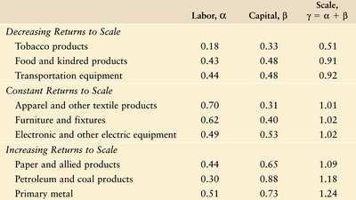
Summary Table: Returns to Scale in U.S. Manufacturing

Type	Labor, α	Capital, β	Scale, γ = α + β
Decreasing Returns to Scale	0.18–0.44	0.33–0.48	0.51–0.92
Constant Returns to Scale	0.49–0.70	0.31–0.53	1.01–1.02
Increasing Returns to Scale	0.30–0.51	0.65–0.88	1.09–1.24

Key Formulas

• Profit: $\pi = R - C$

• Production function: $q = f(L, K)$

• Marginal Product of Labor: $MPL = \frac{\Delta q}{\Delta L}$

• Average Product of Labor: $APL = \frac{q}{L}$

• MRTS: $MRTS = \frac{\Delta K}{\Delta L}$

• Cobb-Douglas: $q = AL^{\alpha}K^{\beta}$

Applications and Examples

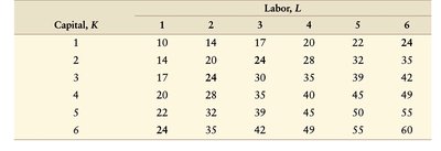
• Tables and figures illustrate how output changes with varying labor and capital, and how returns to scale differ across industries.

• Isoquants and MRTS are used to analyze input substitution and efficiency in production.

Additional info: Academic context and explanations have been expanded for clarity and completeness. All tables and figures included are directly relevant to the microeconomics topics covered in Chapter 6: Firms and Production.