Chapter 7: The Cost of Production – Microeconomics Study Notes

The Cost of Production

Introduction

This chapter explores the theory of production costs, focusing on how firms measure, analyze, and minimize costs in both the short run and long run. Understanding cost structures is essential for firms to make optimal production and pricing decisions.

7.1 Measuring Cost: Which Costs Matter?

Economic Cost vs. Accounting Cost

• Accounting cost: Actual expenses plus depreciation charges for capital equipment.

• Economic cost: The cost to a firm of utilizing economic resources in production, including opportunity costs.

• Opportunity cost: The value of the best alternative use of resources. Economic cost always includes opportunity cost.

Example: Choosing the location for a new law school building should consider the opportunity cost of land, not just explicit expenses.

Sunk Costs

• Sunk cost: An expenditure that has been made and cannot be recovered. Sunk costs should not affect future decisions.

• Prospective sunk costs (investments) should be considered in decision-making before they are incurred.

Fixed and Variable Costs

• Total cost (TC): The sum of fixed and variable costs.

• Fixed cost (FC): Does not vary with output; can only be eliminated by shutting down.

• Variable cost (VC): Varies as output varies.

Marginal and Average Cost

• Marginal cost (MC): The increase in cost from producing one more unit of output.

• Average total cost (ATC): Total cost divided by output.

• Average fixed cost (AFC): Fixed cost divided by output.

• Average variable cost (AVC): Variable cost divided by output.

Formulas:

• $MC = \frac{\Delta TC}{\Delta q} = \frac{\Delta VC}{\Delta q}$

• $ATC = \frac{TC}{q}$

• $AFC = \frac{FC}{q}$

• $AVC = \frac{VC}{q}$

Table: A Firm’s Costs

Output (q)	FC	VC	TC	MC	AFC	AVC	ATC
0	50	0	50	–	–	–	–
1	50	50	100	50	50	50	100
2	50	78	128	28	25	39	64
3	50	98	148	20	16.7	32.7	49.3
4	50	112	162	14	12.5	28	40.5
5	50	130	180	18	10	26	36
6	50	150	200	20	8.3	25	33.3
7	50	175	225	25	7.1	25	32.1
8	50	204	254	29	6.3	25.5	31.8
9	50	242	292	38	5.6	26.9	32.4
10	50	300	350	58	5	30	35
11	50	385	435	85	4.5	35	39.5

7.2 Cost in the Short Run

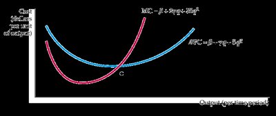
The Shapes of the Cost Curves

• Total cost (TC) is the sum of fixed cost (FC) and variable cost (VC).

• Marginal cost (MC) crosses both the average variable cost (AVC) and average total cost (ATC) at their minimum points.

The Average-Marginal Relationship

• When MC is below ATC or AVC, the average falls; when MC is above, the average rises.

• The vertical distance between ATC and AVC decreases as output increases because AFC declines.

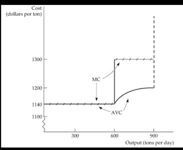
Short-Run Cost Example: Aluminum Smelting

• For output up to 600 tons/day, marginal and average variable costs are constant.

• Beyond 600 tons/day, costs rise sharply due to increased labor, maintenance, and freight costs.

7.3 Cost in the Long Run

User Cost of Capital

• User cost of capital: Annual cost of owning and using a capital asset, equal to economic depreciation plus forgone interest.

• Formula: $\text{User Cost of Capital} = \text{Economic Depreciation} + (\text{Interest Rate}) \times (\text{Value of Capital})$

• Expressed as a rate: $r = \text{Depreciation rate} + \text{Interest rate}$

Cost-Minimizing Input Choice

• Firms choose combinations of labor (L) and capital (K) to minimize cost for a given output.

• The isocost line shows all combinations of L and K that cost the same total amount: $C = wL + rK$

• Slope of isocost line: $-\frac{w}{r}$

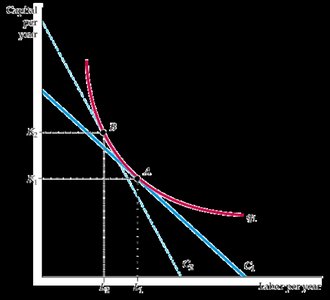
Input Substitution When Input Prices Change

• If the price of labor increases, the isocost line becomes steeper, and the firm substitutes capital for labor to minimize cost.

Cost-Minimizing Condition

• At the cost-minimizing input combination: $\frac{MP_L}{w} = \frac{MP_K}{r}$

• Or equivalently: $\frac{MP_L}{MP_K} = \frac{w}{r}$

Example: Effluent Fees and Input Choices

• Effluent fees increase the cost of using polluting inputs, causing firms to substitute away from them.

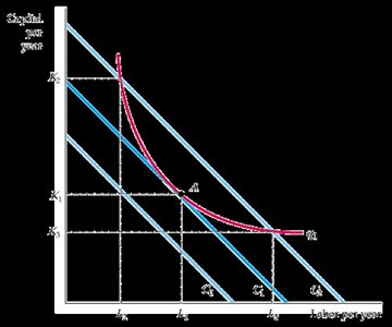
Expansion Path

• The expansion path connects the cost-minimizing combinations of inputs for different output levels.

• It is derived from the tangency points of isocost lines and isoquants.

7.4 Long-Run versus Short-Run Cost Curves

Long-Run Average Cost (LAC) and Marginal Cost (LMC)

• LAC: Average cost when all inputs are variable.

• SAC: Average cost when some inputs (e.g., capital) are fixed.

• LMC: Change in long-run total cost from producing one more unit.

• LMC intersects LAC at its minimum point.

Economies and Diseconomies of Scale

• Economies of scale: Output can be doubled for less than a doubling of cost.

• Diseconomies of scale: Doubling output requires more than double the cost.

• Measured by cost-output elasticity: $EC = \frac{\Delta C / C}{\Delta q / q}$

• If $EC < 1$, economies of scale; if $EC > 1$, diseconomies of scale.

Example: Tesla’s Battery Costs

• Large-scale production at Tesla’s Gigafactory reduces average battery costs due to economies of scale.

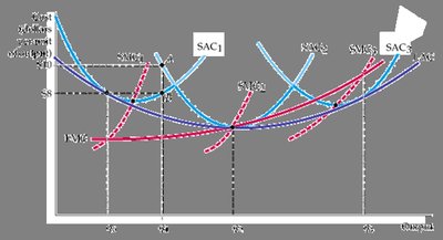
Relationship between Short-Run and Long-Run Cost

• The long-run average cost curve is the envelope of the short-run average cost curves.

7.5 Production with Two Outputs—Economies of Scope

Product Transformation Curves

• Shows combinations of two outputs that can be produced with a fixed set of inputs.

• Bowed-out curves indicate economies of scope.

Economies and Diseconomies of Scope

• Economies of scope: Joint output of a single firm is greater than what two separate firms could achieve.

• Diseconomies of scope: Joint output is less than what could be achieved separately.

• Degree of economies of scope: $SC = \frac{C(q_1, 0) + C(0, q_2) - C(q_1, q_2)}{C(q_1, q_2)}$

Example: Economies of Scope in Trucking

• Large trucking firms can combine loads efficiently, but very large size may reduce scope economies due to management complexity.

7.6 Dynamic Changes in Costs—The Learning Curve

The Learning Curve

• As cumulative output increases, the amount of inputs needed per unit falls due to learning and experience.

• Learning curve equation: $L = A + BN^{-b}$

Learning vs. Economies of Scale

• Learning curve: Cost reductions from accumulated experience.

• Economies of scale: Cost reductions from increased scale of production at a point in time.

Example: Learning Curve in Aircraft Production

• Labor requirements per aircraft decrease as more aircraft are produced, reflecting learning effects.

7.7 Estimating and Predicting Cost

Cost Functions

• Relate cost of production to output and other controllable variables.

• Common forms: Linear ($VC = \beta q$), quadratic ($VC = \beta q + \gamma q^2$), cubic ($VC = \beta q + \gamma q^2 + \delta q^3$).

Scale Economies Index (SCI)

• SCI = 1 − EC, where EC is the cost-output elasticity.

• SCI > 0 indicates economies of scale; SCI < 0 indicates diseconomies.

Example: Cost Functions for Electric Power

• Empirical studies show that average cost in electric power production falls with output up to a point, then rises.

Appendix: Production and Cost Theory—A Mathematical Treatment

Cost Minimization with Two Inputs

• Given a production function $F(K, L)$, minimize $C = wL + rK$ subject to $F(K, L) = q_0$.

• Set up the Lagrangian and solve for the cost-minimizing input combination.

• At the optimum: $\frac{MP_L}{w} = \frac{MP_K}{r}$

Cobb-Douglas Production and Cost Functions

• Production function: $q = A K^{\alpha} L^{\beta}$

• Returns to scale depend on $\alpha + \beta$: constant if $= 1$, increasing if $> 1$, decreasing if $< 1$.

• Cost-minimizing input demands and total cost can be derived using the Lagrangian method.

Example: If the wage rate doubles, the firm substitutes capital for labor to minimize the increase in total cost.

Additional info: These notes include expanded academic context and formulas for clarity and completeness.