Consumer Behaviour: Utility, Demand, and Surplus

Chapter 6: Consumer Behaviour

6a Marginal Utility

Understanding how consumers derive satisfaction from goods is central to microeconomics. This section introduces the concepts of total utility, marginal utility, and the law of diminishing marginal utility.

• Total Utility (TU): The total satisfaction a consumer receives from consuming a certain quantity of a good. Measured in hypothetical units called utils.

• Marginal Utility (MU): The additional satisfaction gained from consuming one more unit of a good. Calculated as: $MU = \frac{\Delta TU}{\Delta Q}$

• Law of Diminishing Marginal Utility: As a consumer consumes more units of a good, the additional satisfaction (marginal utility) from each extra unit decreases, holding all else constant (ceteris paribus).

Example: Brett’s total utility from consuming avocados increases with each additional avocado, but the marginal utility from each extra avocado decreases. This is illustrated in the following graphs:

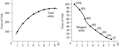
The left graph shows total utility rising at a decreasing rate, while the right graph shows marginal utility declining as quantity increases.

6b Utility Maximization

Consumers aim to allocate their income to maximize total satisfaction. Utility maximization involves two key conditions:

• Condition #1 (Budget Constraint): The consumer spends their entire budget: $P_x Q_x + P_y Q_y = I$ where P is price, Q is quantity, and I is income.

• Condition #2 (Equal Marginal Utility per Dollar): The last dollar spent on each good yields the same marginal utility: $\frac{MU_x}{P_x} = \frac{MU_y}{P_y}$

Example: If MUx = 10, MUy = 7, Px = $1, Py = $2, then:$ \frac{10}{1} = 10 $and$ \frac{7}{2} = 3.5 $. Since these are not equal, the consumer is not maximizing utility. To increase utility, the consumer should buy more of good X and less of good Y until the ratios are equalized.

6c Deriving the Demand Curve

The demand curve shows the relationship between the price of a good and the quantity demanded. Utility maximization explains why demand curves slope downward.

• When the price of good X falls, $\frac{MU_x}{P_x}$ increases, disrupting the utility-maximizing condition.

• The consumer responds by buying more of X (and less of Y), restoring equilibrium. This adjustment process results in a downward-sloping demand curve.

Example: If MUx = 4, MUy = 2, Px = 2, Py = 1, then $\frac{4}{2} = 2$ and $\frac{2}{1} = 2$, so utility is maximized. If Px falls to $1,$ \frac{4}{1} = 4 $, so the consumer will buy more of X.

• Market Demand Curve: The horizontal sum of all individual demand curves. For example, if Yoko’s demand is $Q_Y = 10,000 - 100P$ and Justin’s is $Q_J = 5,000 - 200P$, the market demand is $Q_{total} = Q_Y + Q_J$.

6e Consumer and Producer Surplus

Economic surplus in a market can be divided into consumer and producer surplus, which measure the benefits to buyers and sellers, respectively.

• Consumer Surplus (CS): The difference between what consumers are willing to pay and what they actually pay. Graphically, it is the area under the demand curve and above the market price.

• Producer Surplus (PS): The difference between the market price and the minimum price at which producers are willing to sell. It is the area above the supply curve and below the market price.

• Economic Surplus: The sum of consumer and producer surplus. At equilibrium, it is maximized and equals the area between the demand and supply curves from Q = 0 to Q*.

Example: If equilibrium quantity Q* = 250 units, economic surplus = $3,125.

The Water-Diamond Paradox

This classic paradox asks why water, essential for life, is cheaper than diamonds, which are not essential. The answer lies in marginal utility: water is abundant, so its marginal utility (and price) is low, while diamonds are scarce, so their marginal utility (and price) is high.