Economic Efficiency, Government Price Setting, and Taxes: Study Notes

Economic Efficiency, Government Price Setting, and Taxes

Chapter Overview

This chapter explores how markets allocate resources efficiently, the concepts of consumer and producer surplus, and the effects of government interventions such as price floors, price ceilings, and taxes. It also examines the resulting economic outcomes, including deadweight loss and tax incidence.

Consumer Surplus and Producer Surplus

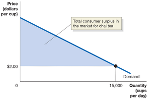
Consumer Surplus

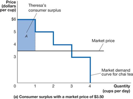
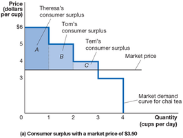
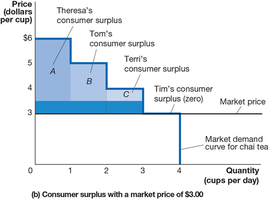
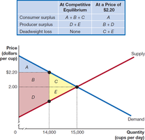
Consumer surplus measures the benefit consumers receive when they pay less for a good than the maximum price they are willing to pay. It is the area below the demand curve and above the market price.

• Definition: The difference between the highest price a consumer is willing to pay and the actual price paid.

• Marginal Benefit: The additional benefit from consuming one more unit of a good or service.

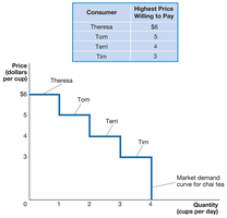
• Graphical Representation: For a market with a few consumers, the demand curve is step-shaped; with many consumers, it becomes a smooth, downward-sloping line.

• Formula (for a linear demand curve): $CS = \frac{1}{2} \times \text{base} \times \text{height}$

• Example: If the price of chai tea is $3.50, and Theresa is willing to pay $6.00, her consumer surplus is $6.00 - $3.50 = $2.50.

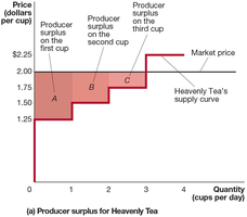
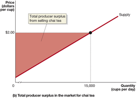
Producer Surplus

Producer surplus is the benefit producers receive when they sell a good for more than the minimum price they are willing to accept, which is typically their marginal cost of production. It is the area above the supply curve and below the market price.

• Definition: The difference between the lowest price a firm would accept and the price it actually receives.

• Marginal Cost: The change in total cost from producing one more unit.

• Formula (for a linear supply curve): $PS = \frac{1}{2} \times \text{base} \times \text{height}$

• Example: If the market price is $2.00 and the marginal cost for the first cup is $1.25, the producer surplus for that cup is $2.00 - $1.25 = $0.75.

Economic Surplus

Economic surplus is the sum of consumer and producer surplus. It is maximized at the competitive market equilibrium, where marginal benefit equals marginal cost.

• Formula: $\text{Economic Surplus} = \text{Consumer Surplus} + \text{Producer Surplus}$

• Efficiency Condition: $MB = MC$ at equilibrium.

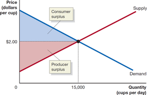
The Efficiency of Competitive Markets

Conditions for Market Efficiency

A market is efficient if all trades where marginal benefit exceeds marginal cost occur, and no trades where marginal cost exceeds marginal benefit take place. At equilibrium, economic surplus is maximized.

• If quantity is too low: $MB > MC$ (shortage, underproduction)

• If quantity is too high: $MB < MC$ (surplus, overproduction)

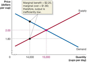
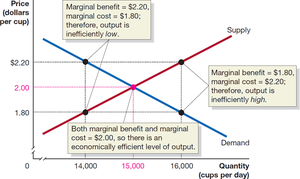
Deadweight Loss

Deadweight loss is the reduction in economic surplus resulting from a market not being in competitive equilibrium. It represents the value of trades that do not occur due to inefficiency.

• Formula: $\text{Deadweight Loss} = \text{Lost Consumer Surplus} + \text{Lost Producer Surplus}$

Government Intervention: Price Floors and Price Ceilings

Price Floors

A price floor is a legally established minimum price. It is only effective if set above the equilibrium price. Common examples include minimum wage and agricultural price supports.

• Creates a surplus (excess supply) if binding.

• Transfers surplus from consumers to producers but creates deadweight loss.

Price Ceilings

A price ceiling is a legally established maximum price. It is only effective if set below the equilibrium price. Common examples include rent control.

• Creates a shortage (excess demand) if binding.

• Transfers surplus from producers to consumers but creates deadweight loss.

Economic Effects of Price Controls

• Winners: Those who can buy at the lower price (price ceiling) or sell at the higher price (price floor).

• Losers: Those who cannot find the good (shortage) or cannot sell the good (surplus).

• Always results in a loss of economic efficiency (deadweight loss).

The Economic Effect of Taxes

Types of Taxes

• Per-Unit Tax: A fixed amount charged on each unit sold (e.g., excise tax).

• Percentage Tax: A percentage of the price (e.g., sales tax).

Tax Incidence

Tax incidence refers to the actual division of the burden of a tax between buyers and sellers, regardless of who is legally responsible for paying the tax.

• Determined by the relative elasticities (slopes) of demand and supply.

• If demand is inelastic (steep), consumers bear more of the tax burden.

• If supply is inelastic (steep), producers bear more of the tax burden.

Effects of a Tax on Market Outcomes

• Shifts the supply curve upward by the amount of the tax (if imposed on sellers) or the demand curve downward (if imposed on buyers).

• Reduces the equilibrium quantity traded.

• Creates deadweight loss (excess burden).

• Generates tax revenue for the government.

Calculating Tax Revenue and Deadweight Loss

• Tax Revenue: $\text{Tax Revenue} = \text{Tax per unit} \times \text{Quantity sold after tax}$

• Deadweight Loss: $\text{Deadweight Loss} = \frac{1}{2} \times \text{Tax per unit} \times \text{Reduction in quantity sold}$

Example: Tax on Cigarettes

• Without tax: Equilibrium price is $6.00, quantity is 4 billion packs.

• With $1.00 tax: Supply shifts up, new equilibrium price is $6.90, quantity is 3.7 billion packs.

• Producers receive $5.90 after tax.

• Tax revenue is the area of the green box; deadweight loss is the yellow triangle.

Example: Tax Incidence on Gasoline

• With a $0.10 per-gallon tax, price rises from $2.50 to $2.58 for consumers, falls to $2.48 for sellers.

• Consumers pay $0.08, sellers pay $0.02 of the tax.

Social Security Tax Example

• FICA tax is split legally between employers and workers, but the burden falls mostly on workers due to inelastic labor supply.

Summary Table: Effects of Rent Controls (Appendix Example)

Scenario	Consumer Surplus	Producer Surplus	Deadweight Loss
Before Rent Control	$2,531.25 million	$1,947.375 million	$0
After Rent Control	Increases by area A, loses area B	Loses area A and C	$1,495 million

Additional info: The appendix provides quantitative tools for calculating equilibrium, surplus, and deadweight loss using demand and supply equations. These calculations reinforce the graphical and conceptual analysis presented in the main chapter.