Firms in Perfectly Competitive Markets: Microeconomics Study Notes

Firms in Perfectly Competitive Markets

Market Structures and the Four Market Models

Market structure refers to the environment in which firms operate, primarily determined by the number of firms, the nature of the product, and barriers to entry. The four main market models are:

• Perfect Competition

• Monopolistic Competition

• Oligopoly

• Monopoly

Each model differs in terms of the number of firms, product differentiation, barriers to entry, and the relationship between price, marginal revenue, and marginal cost.

Characteristics of Perfect Competition

A perfectly competitive market is defined by several key characteristics:

• Homogeneous Goods: The goods for sale are identical or standardized.

• Price Takers: Both buyers and sellers have no influence over the market price; they accept the market price as given.

• Many Buyers and Sellers: There are numerous participants on both sides of the market.

• Free Entry and Exit: Firms can freely enter or exit the market in the long run.

• Example Product: Agricultural products like wheat are classic examples.

The demand curve facing an individual firm is perfectly elastic (horizontal), while the market demand curve is downward sloping.

Revenue in Perfect Competition

Revenue is the income a firm receives from selling its product. In perfect competition:

• Total Revenue (TR): The total income from sales, calculated as $TR = P \times Q$.

• Average Revenue (AR): Revenue per unit sold, $AR = \frac{TR}{Q}$.

• Marginal Revenue (MR): The additional revenue from selling one more unit, $MR = \frac{\Delta TR}{\Delta Q}$.

• In perfect competition, $AR = MR = P$ because the price is constant for each unit sold.

Example: If the market price per bushel of wheat is $4, then selling each additional bushel always adds $4 to total revenue.

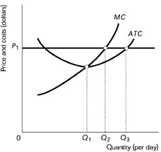
Profit Maximization in Perfect Competition

The profit-maximizing quantity for a perfectly competitive firm occurs where marginal revenue equals marginal cost ($MR = MC$). The profit or loss is calculated as:

• $Profit = (P - ATC) \times Q$

Steps to find profit-maximizing output:

1. Find the quantity where $MR = MC$.

2. Determine the price (from the demand curve) and average total cost (ATC) at that quantity.

Interpretation:

• If $P > ATC$, the firm earns an economic profit.

• If $P = ATC$, the firm breaks even (zero economic profit).

• If $P < ATC$, the firm incurs an economic loss.

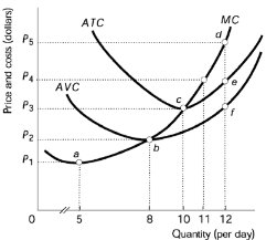
Short-Run Shutdown Decision

In the short run, a firm may decide to temporarily shut down if market conditions are unfavorable. Key points:

• Shutdown: The firm produces no output temporarily but remains in the market.

• Exit: The firm leaves the market permanently.

• Sunk Cost: A cost that cannot be recovered (e.g., a non-refundable lease payment).

• The relevant cost for shutdown is the average variable cost (AVC).

• The shutdown point is the minimum of the AVC curve.

Shutdown rule:

• Shutdown if $P < AVC$

• Produce if $P > AVC$

Summary Table:

Should firm produce?	Yes, if $P > AVC$	No, if $P < AVC$
If yes, what quantity?	Produce where $MR = MC$
Economic profit?	Yes, if $P > ATC$	No, if $P < ATC$

Long-Run Exit and Entry Decisions

In the long run, firms can enter or exit the market. The relevant cost is the average total cost (ATC):

• Exit if $P < ATC$ (cannot cover all costs)

• Enter if $P > ATC$ (profit opportunity exists)

• In the long run, all costs are variable and there are no sunk costs.

• The minimum of the ATC curve is the entry/exit point.

Individual and Market Supply Curves

The supply curve for a perfectly competitive firm is determined by its marginal cost curve:

• Short-Run Supply Curve: The portion of the MC curve above the AVC curve.

• Long-Run Supply Curve: The portion of the MC curve above the ATC curve.

The market supply curve is the horizontal sum of all individual firms' supply curves. In the short run, the number of firms is fixed; in the long run, entry and exit drive economic profit to zero.

Changes in Demand and Long-Run Equilibrium

Shifts in the demand curve can create short-run profits or losses, but in the long run, entry and exit of firms return the market to zero economic profit (long-run equilibrium).

• Short-run: Firms can earn profits or losses.

• Long-run: Entry or exit of firms restores zero economic profit.

Perfect Competition and Efficiency

Perfect competition achieves both productive and allocative efficiency:

• Productive Efficiency: Producing at the lowest possible cost (minimum ATC).

• Allocative Efficiency: Producing the quantity where price equals marginal cost ($P = MC$), ensuring resources are allocated to their most valued use.

In perfect competition, $P = MB = MC$, where MB is the marginal benefit to consumers.

Summary Table: The Four Market Models

Market Structure	Number of Firms	Examples	Barriers to Entry	Profit-Maximizing Quantity	Long-Run Profitability	Relation of Price (P=AR) and MR	Relation of Price and MC
Perfect Competition	Many	Agricultural products	None	$MR = MC$	Zero economic profit	$P = AR = MR$	$P = MC$
Monopolistic Competition	Many	Retail clothing	Low	$MR = MC$	Zero economic profit	$P > MR$	$P > MC$
Oligopoly	Few	Automobiles	High	$MR = MC$	Possible profit	$P > MR$	$P > MC$
Monopoly	One	Utilities	Very high	$MR = MC$	Possible profit	$P > MR$	$P > MC$

Practice Questions and Applications

• Practice questions throughout the notes reinforce understanding of profit maximization, shutdown decisions, and long-run equilibrium.

• Graphical analysis is essential for visualizing cost curves, profit areas, and market adjustments.