 Back
BackHousehold Behavior and Consumer Choice: Budget Constraints and Utility
Study Guide - Smart Notes
 Tailored notes based on your materials, expanded with key definitions, examples, and context.
Household Behavior and Consumer Choice
Introduction to Household Choices
Households face fundamental tradeoffs in their economic decisions, balancing consumption, labor supply, and savings. These choices are constrained by limited resources and are central to understanding microeconomic behavior in output, labor, and financial markets.
Key Point 1: Households must decide how much of each product to demand, how much labor to supply, and how much to spend versus save.
Key Point 2: Every decision involves opportunity costs, as increasing consumption of one good or activity reduces the ability to consume others.
Example: Working more hours increases income and consumption but reduces leisure time.
Household Choice in Output Markets
Budget Constraint: What the Consumer Can Afford
The budget constraint represents the combinations of goods a consumer can purchase given their income and the prices of goods. It defines the consumer's opportunity set and limits their choices.
Key Point 1: A consumption bundle is a specific combination of goods (e.g., 40 fish & 300 mangos).
Key Point 2: The budget constraint is mathematically expressed as: , where and are prices of fish and mangos, and , are their quantities.
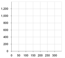
Example: If Hurley has $1200, fish cost $4, and mangos $1, he can buy 300 fish or 1200 mangos, or any combination in between.
Graphical Representation of the Budget Constraint
The budget constraint can be visualized on a graph with one good on each axis. The slope of the constraint reflects the opportunity cost of one good in terms of the other.
Key Point 1: The slope is calculated as the negative ratio of the prices: .
Key Point 2: Moving along the constraint, the consumer must give up units of one good to gain units of the other.
Example: Hurley must give up 4 mangos to get one fish, so the slope is -4.
Opportunity Set and Effects of Changes in Income and Prices
The opportunity set is the collection of all affordable bundles. Changes in income or prices shift or pivot the budget constraint, altering the opportunity set.
Key Point 1: A decrease in income shifts the budget constraint inward, reducing the opportunity set.
Key Point 2: An increase in the price of one good pivots the constraint inward, changing the slope and opportunity cost.
Example: If Hurley's income falls to $800, he can buy fewer fish and mangos. If the price of mangos rises to $2, he can buy fewer mangos for the same income.
Utility: The Basis of Consumer Choice
Definitions and Concepts
Utility measures the satisfaction a consumer derives from consuming goods and services. Total utility is the overall satisfaction, while marginal utility is the additional satisfaction from consuming one more unit.
Key Point 1: Utility is the happiness or satisfaction from a product.
Key Point 2: Total utility is the sum of satisfaction from all units consumed; marginal utility (MU) is the extra satisfaction from one additional unit.
Example: Eating a second chocolate bar yields less additional satisfaction than the first.
Diminishing Marginal Utility
The law of diminishing marginal utility states that as more of a good is consumed, the additional satisfaction from each extra unit decreases. This principle explains why consumers diversify their consumption.
Key Point 1: Marginal utility decreases with each additional unit consumed.
Key Point 2: This leads to downward-sloping demand curves, as consumers are willing to pay less for additional units.
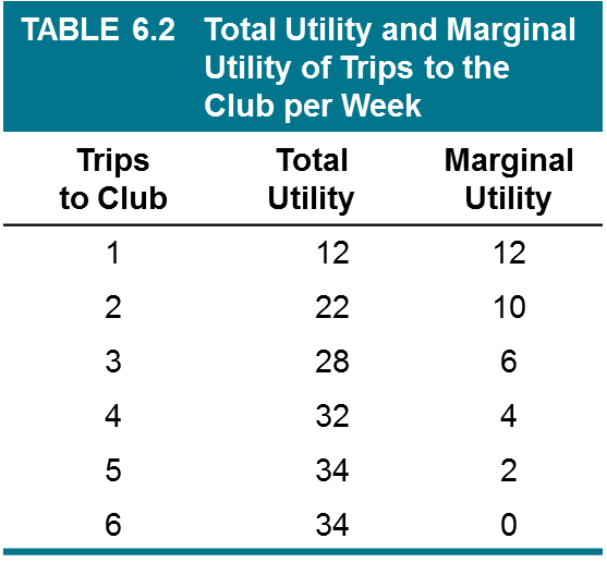
Example: The utility from the second trip to the club is less than from the first.

Utility-Maximizing Rule
Consumers allocate their income to maximize utility by equating the ratio of marginal utility to price across all goods. This ensures the last dollar spent on each good yields equal satisfaction.
Key Point 1: The utility-maximizing rule is: .
Key Point 2: If the ratio is not equal, the consumer should adjust consumption to increase total utility.
Example: If , consume more of Y and less of X.
Table: Total Utility and Marginal Utility
The following table illustrates how total utility and marginal utility change with the number of trips to the club per week.
Trips per Week | Total Utility | Marginal Utility |
|---|---|---|
1 | 20 | 20 |
2 | 38 | 18 |
3 | 54 | 16 |
4 | 68 | 14 |
5 | 80 | 12 |
6 | 90 | 10 |
7 | 98 | 8 |
Diminishing Marginal Utility and Demand
Connection to Demand Curves
Diminishing marginal utility explains why demand curves slope downward. As consumers buy more of a good, the additional satisfaction decreases, so they are willing to pay less for extra units.
Key Point 1: Consumers spread their income over a variety of goods to maximize utility.
Key Point 2: The downward slope of demand curves reflects diminishing marginal utility.
