Intermediate Microeconomics: Competitive Markets, Government Intervention, Monopoly, Oligopoly, and Game Theory

Perfect Competition

Characteristics of Perfectly Competitive Markets

Perfect competition is an idealized market structure that provides a benchmark for understanding market forces. It is characterized by:

• Many buyers and sellers: No single agent can influence the market price.

• Identical products: Goods are perfect substitutes.

• Perfect information: All participants know prices and product characteristics.

• Equal access to resources: No firm has a permanent advantage.

• Price takers: Firms and consumers accept the market price.

• Law of one price: Identical goods sell for the same price everywhere.

• Free entry and exit: Firms can enter or leave the market freely, driving long-run profit to zero.

Examples: Agricultural and commodity markets (e.g., wheat, crude oil) approximate perfect competition.

Economic vs. Accounting Profit

• Accounting profit: Revenue minus explicit costs.

• Economic profit: Revenue minus explicit costs and opportunity costs.

• Opportunity cost: The value of the next best alternative forgone.

Zero economic profit means earning as much as in the next best alternative, not necessarily making a loss.

Profit Maximization Rule

• Golden Rule: Produce where marginal revenue (MR) equals marginal cost (MC).

• In perfect competition, MR = P, so the rule simplifies to P = MC (on the upward-sloping part of MC).

Short-Run Cost Concepts

• Total Cost (TC): $TC = TFC + TVC$

• Average Cost (AC): $AC = TC / Q$

• Average Variable Cost (AVC): $AVC = TVC / Q$

• Average Fixed Cost (AFC): $AFC = TFC / Q$

• Marginal Cost (MC): $MC = dTC/dQ$

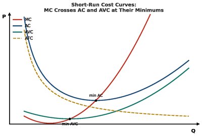
Key property: MC crosses both AC and AVC at their minimum points.

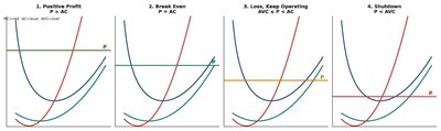
The Four Short-Run Cases

1. Positive profit: $P > AC$

2. Break even: $P = AC$

3. Loss, keep operating: $AVC \leq P < AC$

4. Shutdown: $P < AVC$

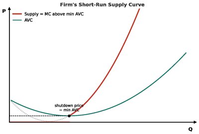
Short-Run Supply Curve

• The firm's short-run supply curve is the upward-sloping part of the MC curve above the shutdown price (minimum AVC).

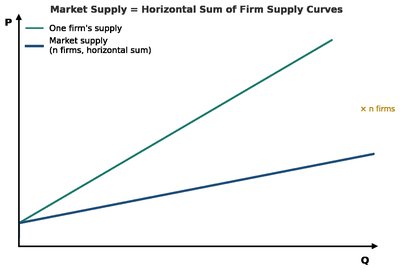
Market Supply Curve

• The market supply curve is the horizontal sum of all individual firms' supply curves.

Short-Run Market Equilibrium

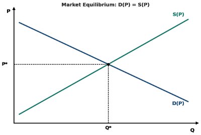
• Equilibrium price and quantity are found where market demand equals market supply: $D(P^*) = S(P^*)$.

Long-Run Equilibrium

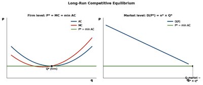
• In the long run, entry and exit drive economic profit to zero.

• All firms produce at the minimum point of their AC curve: $P^* = MC(Q^*) = min AC(Q^*)$.

• Market clears: $D(P^*) = n^* \times Q^*$.

Long-Run Market Supply Curve

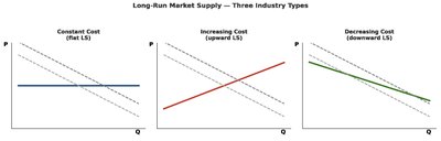
• The shape depends on input cost changes as industry expands:

Industry Type	Input Costs	LR Supply Curve
Constant cost	Unchanged	Horizontal
Increasing cost	Rise	Upward sloping
Decreasing cost	Fall	Downward sloping

Producer Surplus (PS)

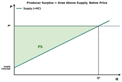
• Producer surplus is the area above the supply curve and below the market price.

• For a linear supply curve: $PS = \frac{1}{2} (P^* - \text{price intercept}) Q^*$

Government Intervention in Competitive Markets

Surplus and Efficiency

• Consumer surplus (CS): Value buyers receive above what they pay.

• Producer surplus (PS): Value sellers receive above their cost.

• Total surplus: $CS + PS$, maximized at market equilibrium.

Deadweight Loss (DWL)

• DWL is the loss in total surplus when market quantity deviates from the efficient level due to intervention.

Excise Taxes

• A per-unit tax shifts the supply curve up by the tax amount.

• Creates a wedge: $P_d = P_s + t$

• Reduces quantity traded, raises price for consumers, lowers price for producers.

• DWL: $\frac{1}{2} \times |\Delta Q| \times t$

Tax Incidence

• The side of the market (buyers or sellers) that is less elastic bears more of the tax burden.

• Incidence ratio: $\frac{\Delta P_{consumer}}{\Delta P_{producer}} = \frac{E_{supply}}{E_{demand}}$

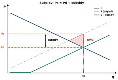
Subsidies

• A per-unit subsidy shifts the supply curve down by the subsidy amount.

• Increases quantity traded, lowers price for consumers, raises price for producers.

• DWL: $\frac{1}{2} \times |\Delta Q| \times \text{subsidy}$

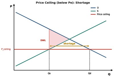
Price Ceilings

• A legal maximum price set below equilibrium creates a shortage (quantity demanded exceeds quantity supplied).

• Results in DWL and possible misallocation of goods.

Price Floors

• A legal minimum price set above equilibrium creates a surplus (quantity supplied exceeds quantity demanded).

• Results in DWL and possible misallocation of resources.

Monopoly and Monopsony

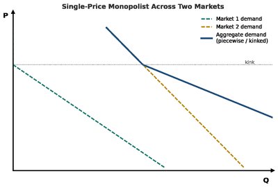
Monopoly: Key Features

• A single firm supplies the entire market and faces the downward-sloping market demand curve.

• Profit maximization: $MR = MC$

• Marginal revenue is always less than price for positive output: $MR = P + Q \cdot (dP/dQ)$

• No supply curve exists for a monopolist.

Inverse Elasticity Pricing Rule (IEPR)

• Optimal markup: $\frac{P - MC}{P} = -\frac{1}{\varepsilon}$, where $\varepsilon$ is the price elasticity of demand.

• More elastic demand leads to a lower markup.

Lerner Index

• Measures market power: $L = \frac{P - MC}{P}$

• Ranges from 0 (perfect competition) to 1 (maximum market power).

Elastic vs. Inelastic Demand

• A monopolist always operates on the elastic portion of the demand curve ($\varepsilon < -1$).

Multi-Plant Monopoly

• Optimal allocation: $MC_1 = MC_2 = MR$

• Production is shifted toward the lower-cost plant.

Monopsony

• A single buyer faces an upward-sloping supply curve and must pay higher prices to attract more units.

• Optimal hiring: $MRPL = MEL$ (Marginal Revenue Product of Labour equals Marginal Expense of Labour).

• Wage paid is read off the supply curve at $L^*$.

Oligopoly and Game Theory

Cournot Model (Quantity Competition)

• Firms choose quantities simultaneously; each firm's output affects market price.

• Best response functions determine equilibrium output for each firm.

• As the number of firms increases, the outcome approaches perfect competition.

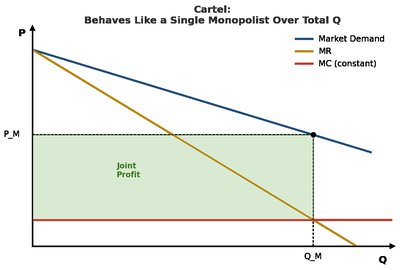
Cartel (Collusion)

• Firms act together as a monopolist to maximize joint profit, restricting output and raising price.

Bertrand Model (Price Competition)

• Firms choose prices simultaneously; with homogeneous products, price is driven down to marginal cost (Bertrand Paradox).

Stackelberg Model (Sequential Quantities)

• One firm (leader) chooses output first; the follower observes and responds.

• Leader earns higher profit due to first-mover advantage.

Dominant Firm Model

• One large firm sets price; many small firms act as price takers.

• Dominant firm faces residual demand after accounting for the fringe supply.

Product Differentiation

• Vertical differentiation: products differ in quality.

• Horizontal differentiation: products differ in characteristics or style.

• Differentiation softens price competition, allowing positive profits.

Game Theory

Nash Equilibrium

• A set of strategies where no player can improve their payoff by unilaterally changing their strategy.

• Can be found using best response analysis in payoff matrices.

Dominant and Dominated Strategies

• Dominant strategy: Best regardless of what others do.

• Dominated strategy: Worse regardless of what others do; can be eliminated.

Prisoner's Dilemma

• Both players have a dominant strategy leading to a worse outcome than mutual cooperation.

Games with Multiple Nash Equilibria

• Coordination games: players want to match actions (e.g., bank run).

• Anti-coordination games: players want to choose opposite actions (e.g., game of chicken).

Pure vs. Mixed Strategies

• Pure strategy: Always choose the same action.

• Mixed strategy: Randomize between actions to keep opponents indifferent.

Repeated and Sequential Games

• Infinitely repeated games: Cooperation can be sustained if players are patient (high discount factor $\delta$).

• Grim trigger strategy: Cooperate until someone cheats, then defect forever.

• Sequential games: Players move in order; solved by backward induction.

Key Formulas and Concepts

• Profit maximization (all structures): $MR = MC$

• Perfect competition: $P = MC$

• Producer surplus (linear): $PS = \frac{1}{2} (P^* - \text{intercept}) Q^*$

• Tax incidence: $\frac{\Delta P_{consumer}}{\Delta P_{producer}} = \frac{E_{supply}}{E_{demand}}$

• IEPR (monopoly): $\frac{P - MC}{P} = -\frac{1}{\varepsilon}$

• Lerner Index: $L = \frac{P - MC}{P}$

• Cournot output (n firms): $Q^* = \frac{1}{n+1} \frac{A - c}{B}$

• Grim trigger cooperation condition: $\delta > \frac{X - C}{X - P}$