Markets for Factors of Production: The Labor Market

Markets for Factors of Production

Introduction to Labor Markets

The labor market is a fundamental component of microeconomics, where individuals supply labor and firms demand labor services to produce goods and services. The wage rate is the price of labor, determined by the interaction of supply and demand in competitive markets.

• Labor services: The physical and mental work effort supplied by people.

• Labor market: The collection of buyers (firms) and sellers (workers) trading labor services.

• Wage rate: The price paid for labor services, typically expressed per hour.

• Most labor markets are competitive, with many buyers and sellers.

Demand for Labor

Marginal Revenue Product of Labor (MRPL)

Firms decide how much labor to hire based on the additional revenue generated by each worker, known as the Marginal Revenue Product of Labor (MRPL).

• MRPL: The change in total revenue from hiring one more unit of labor.

• Formula: $ MRPL = \frac{\text{Change in Total Revenue}}{\text{Change in Labor}} $

• In a competitive market: $ MRPL = \text{Price} \times \text{Marginal Product of Labor} $

Profit Maximization and Labor Demand

A profit-maximizing firm hires workers up to the point where the MRPL equals the wage rate.

• Hire workers as long as $ MRPL > \text{Wage} $.

• Profit-maximizing condition: $ MRPL = \text{Wage Rate} $

Example Table: Marginal Product and MRPL

Labor (workers)	Output (Hourly)	Marginal Product	Marginal Revenue Product
1	5	5	$50
2	10	5	$50
3	14	4	$40
4	17	3	$30
5	19	2	$20
6	20	1	$10

Example: If the wage rate is $20/hour, the firm hires 5 workers. If the wage is $30/hour, the firm hires 4 workers.

Labor Demand Curve

The firm's demand curve for labor is the same as its MRPL curve. The market demand for labor is the horizontal sum of all firms' labor demand curves.

• The demand for labor depends on the marginal product of labor and the price of the product.

• Formula: $ \text{Marginal Revenue Product} = \text{Marginal Product} \times \text{Price of the Good} $

Shifts in Labor Demand

• Price of Output: Higher output prices increase labor demand (shifts demand curve right).

• Prices of Other Factors: Changes in the cost of capital or materials can affect labor demand.

• Technology: New technology can increase or decrease demand for certain types of labor.

Example: Automation in bakeries reduces demand for bakery workers but increases demand for machine technicians.

Supply of Labor

Individual Labor Supply Decisions

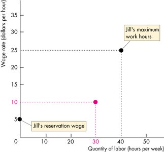
Individuals allocate their time between labor and leisure. The decision to supply labor depends on the wage rate and the individual's reservation wage (the minimum wage at which they are willing to work).

• Reservation wage: The lowest wage rate at which a person is willing to supply labor.

• As the wage rises above the reservation wage, more labor is supplied.

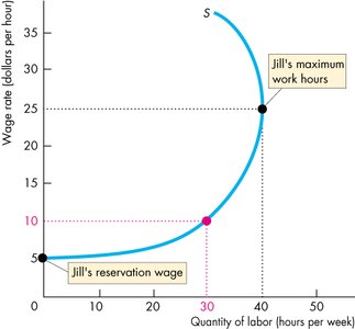
Individual Labor Supply Curve

The supply curve shows the relationship between the wage rate and the quantity of labor supplied by an individual. It may bend backward at high wage rates due to the income effect.

• At low wage rates, higher wages increase labor supplied (substitution effect dominates).

• At high wage rates, higher wages may decrease labor supplied (income effect dominates).

Substitution and Income Effects

• Substitution effect: As wages rise, the opportunity cost of leisure increases, so individuals supply more labor.

• Income effect: As wages rise, income increases, allowing individuals to afford more leisure, so they may supply less labor.

Backward-bending supply curve: At low wages, substitution effect dominates; at high wages, income effect dominates, causing the supply curve to bend backward.

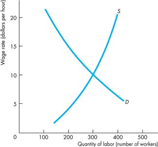
Market Supply of Labor

The market supply curve is the horizontal sum of all individual labor supply curves. It generally slopes upward, even if individual curves bend backward.

• Market supply reflects the total quantity of labor supplied at each wage rate in a particular job market.

Labor Market Equilibrium

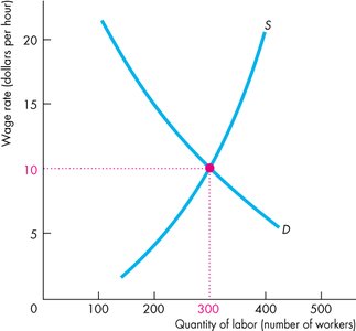
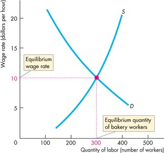
Competitive Labor Market Equilibrium

Equilibrium in the labor market is determined by the intersection of the market demand and supply curves. This equilibrium sets the wage rate and the number of workers employed.

Wage Differentials

Explaining Wage Differences

Wages differ across occupations due to differences in required skills, education, and the cost of acquiring human capital. Occupations requiring more training and higher reservation wages tend to pay more.

• Surgeons earn much more than fast-food workers due to higher training costs and reservation wages.

• Supply curves differ across occupations, reflecting differences in required skills and willingness to work at various wage rates.

Examples of Wage Differentials

Occupation	Hourly Wage	Annual Salary
Fast Food Worker	$18.57	$35,654
Construction Worker	$24	$46,000
Plumber	$33.97	$65,000
Windmill Technician	$31.17	$64,000
Bachelor's Degree (avg.)	-	$77,000
Master's Degree (avg.)	-	$90,324
Economics (median)	-	$107,000
Petroleum Engineer (median)	-	$137,000
Lawyer (NYC, median)	-	$212,000
Orthopaedic Surgeon (median)	-	$466,000

Practice Problems and Applications

Marginal Product and Hiring Decisions

Example: The Red Brick Company produces bricks in a competitive market. Each pound of bricks sells for $20, and the wage rate is $30/hour.

• Marginal product of the fourth worker: 2 pounds/hour

• Value of marginal product: $40/hour

• Optimal hiring: 4 workers, producing 21 pounds/hour

Substitution and Income Effects in Practice

Example: Teddy receives an 8% wage increase but chooses to work fewer hours (from 30 to 25 per week). The opportunity cost of leisure has increased, but the income effect dominates, so Teddy consumes more leisure.

• Opportunity cost of leisure increases with wage.

• If income effect > substitution effect, labor supplied decreases as wage rises.