Microeconomics ECS2601: Core Study Notes

Introduction to Microeconomics

Microeconomics studies the behavior of individual consumers, firms, and markets. It focuses on how resources are allocated, how prices are determined, and how economic agents interact within various market structures. The ECS2601 module covers foundational and intermediate topics essential for understanding microeconomic theory and its applications.

Elasticity

Types of Elasticity

Elasticity measures the responsiveness of one variable to changes in another variable, commonly price or income. It is a critical tool for analyzing demand and supply.

• Price Elasticity of Demand (Ep): Measures the percentage change in quantity demanded resulting from a 1% change in price. Typically negative, but the absolute value is used for interpretation.

• Income Elasticity of Demand: Measures the responsiveness of quantity demanded to changes in consumer income. Positive for normal goods, negative for inferior goods.

• Cross-Price Elasticity of Demand: Measures the responsiveness of demand for one good to changes in the price of another good. Positive for substitutes, negative for complements.

• Price Elasticity of Supply: Measures the responsiveness of quantity supplied to changes in price, usually positive.

Formulas:

• Point Elasticity: $E_p = \frac{dQ}{dP} \times \frac{P}{Q}$

• Arc Elasticity: $E_p = \frac{\Delta Q}{\Delta P} \times \frac{P_1 + P_2}{Q_1 + Q_2}$

Applications: Elasticity helps predict the effects of price changes, taxation, and government interventions such as price floors and ceilings.

Consumer Behaviour

Consumer Preferences and Utility

Consumers make choices to maximize their satisfaction (utility) given their preferences and budget constraints. Preferences are assumed to be complete, transitive, and that more is preferred to less. Utility can be represented by indifference curves, which show combinations of goods yielding the same satisfaction.

• Indifference Curve: Downward sloping and convex to the origin, representing diminishing marginal rate of substitution (MRS).

• Marginal Rate of Substitution (MRS): The rate at which a consumer is willing to trade one good for another, holding utility constant. $MRS_{xy} = -\frac{dY}{dX}$ along an indifference curve.

Budget Constraints

The budget line represents all combinations of goods a consumer can afford given their income and the prices of goods.

• Equation: $P_x X + P_y Y = I$

• Slope: $-\frac{P_x}{P_y}$

Consumer Equilibrium

Equilibrium is reached where the highest attainable indifference curve is tangent to the budget line, i.e., where $MRS = \frac{P_x}{P_y}$.

Marginal Utility and Consumer Choice

Consumers allocate their budget so that the marginal utility per rand spent is equalized across all goods:

• $\frac{MU_x}{P_x} = \frac{MU_y}{P_y}$

Example Table:

Bundle	MU of peanut butter	MU of tuna	Marginal Rate of Substitution
A	0.25	2.41
B	0.31	1.50
C	0.42	0.84
D	0.66	0.33

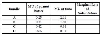
Additional info: The marginal rate of substitution (MRS) between peanut butter and tuna at each bundle can be calculated as $MRS = \frac{MU_{peanut\ butter}}{MU_{tuna}}$.

Production Theory

Production Functions

The production function shows the maximum output that can be produced with given inputs and technology. For two inputs (capital K and labour L):

• $q = F(K, L)$

Short run: At least one input is fixed (usually capital). Long run: All inputs are variable.

Isoquants

Isoquants are curves showing all combinations of inputs that yield the same output, analogous to indifference curves in consumer theory.

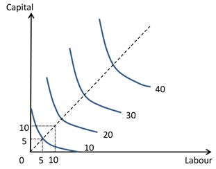
• Marginal Rate of Technical Substitution (MRTS): The rate at which one input can be substituted for another, holding output constant. $MRTS_{LK} = -\frac{dK}{dL} = \frac{MP_L}{MP_K}$

Returns to Scale

• Increasing Returns to Scale: Output increases by a greater proportion than inputs.

• Constant Returns to Scale: Output increases in the same proportion as inputs.

• Decreasing Returns to Scale: Output increases by a smaller proportion than inputs.

The Cost of Production

Short-Run and Long-Run Costs

Cost curves describe the relationship between output and the costs of production. In the short run, some inputs are fixed; in the long run, all inputs are variable.

• Total Cost (TC): $TC = FC + VC$

• Average Cost (AC): $AC = \frac{TC}{q}$

• Marginal Cost (MC): $MC = \frac{\Delta TC}{\Delta q}$

• Average Variable Cost (AVC): $AVC = \frac{VC}{q}$

• Average Fixed Cost (AFC): $AFC = \frac{FC}{q}$

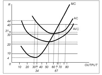
Key relationships: MC intersects AC and AVC at their minimum points. As output increases, AFC declines.

Long-Run Costs

In the long run, firms can adjust all inputs. The long-run average cost curve (LRAC) is typically U-shaped and is the envelope of all possible short-run average cost curves (SRAC).

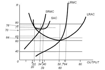
Economies of Scale: LRAC decreases as output increases. Diseconomies of Scale: LRAC increases as output increases.

Summary Table: Key Cost Concepts

Cost Concept	Definition
Economic Cost	Explicit + implicit (opportunity) costs
Accounting Cost	Explicit costs only
Sunk Cost	Past expenditure that cannot be recovered
Marginal Cost (MC)	Change in total cost from producing one more unit
Average Cost (AC)	Total cost divided by output

Conclusion

This guide covers the foundational concepts of microeconomics, including elasticity, consumer behavior, production, and cost theory. Mastery of these topics is essential for analyzing market outcomes, firm decisions, and the effects of government intervention. For further study, refer to the recommended textbook and additional readings provided in the course materials.