Microeconomics Study Guide: Costs, Supply, Surplus, and Externalities

Firms and Production

Production Function and Inputs

The production function describes the relationship between inputs and outputs in a firm. In microeconomics, the most common inputs are labor and capital. The production function is typically written as:

• q = f(L, K): where q is output, L is labor, and K is capital.

• Isoquant Curve: A set of input bundles that generate the same amount of output.

• Isoquant Map: A collection of isoquant curves representing different output levels.

In the short run, some inputs are fixed (e.g., capital), while others are adjustable (e.g., labor). In the long run, all inputs are adjustable.

Costs

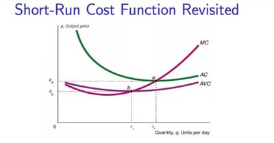
Short-Run Cost Functions

Short-run cost functions are derived based on the fixed and variable inputs:

• Fixed Cost (FC): Cost associated with fixed inputs (e.g., capital).

• Variable Cost (VC): Cost associated with variable inputs (e.g., labor).

• Total Cost (TC): $TC(q) = VC(q) + FC$

• Marginal Cost (MC): $MC(q) = \Delta TC(q) / \Delta q = \Delta VC(q) / \Delta q$

• Average Cost (AC): $AC(q) = TC(q) / q$

• Average Variable Cost (AVC): $AVC(q) = VC(q) / q$

• Average Fixed Cost (AFC): $AFC(q) = FC / q$

Typical properties include U-shaped AC and AVC curves, and MC intersecting AC and AVC at their minimum points.

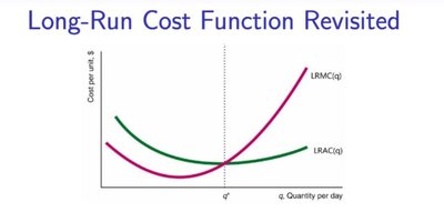
Long-Run Cost Functions

In the long run, all inputs are variable, and the cost functions reflect this flexibility:

• Long-Run Cost Function (LRC): Relationship between target output and minimal cost.

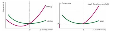
• Long-Run Average Cost (LRAC): $LRAC(q) = LRC(q) / q$

• Long-Run Marginal Cost (LRMC): The extra cost of producing one more unit in the long run.

The LRAC curve is typically U-shaped, reflecting economies and diseconomies of scale. The relationship between LRMC and LRAC is:

• When $q < q^*$: $LRMC < LRAC$

• When $q = q^*$: $LRMC = LRAC$

• When $q > q^*$: $LRMC > LRAC$

Supply Curves

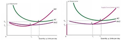
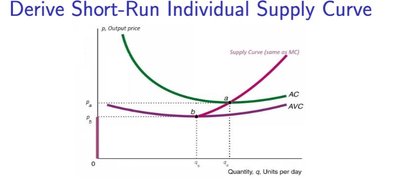
Short-Run Individual Supply Curve

The short-run individual supply curve is the portion of the MC curve above the AVC curve. Producers only supply if the price is above the shut-down price ($p_b$).

• If $p < p_b$: Producer shuts down.

• If $p \geq p_a$: Producer produces until $MR = MC$.

• If $p_b \leq p < p_a$: Producer still produces, but net profit may be negative.

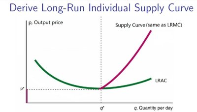
Long-Run Individual Supply Curve

The long-run individual supply curve is the portion of the LRMC curve above the LRAC curve. In the long run, producers can freely enter and exit the market.

• If $p < p^*$: Producer shuts down.

• If $p \geq p^*$: Producer produces until $MR = LRMC$.

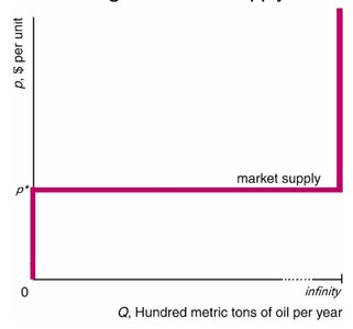
Market Supply Curve

The market supply curve is the sum of individual supply curves:

• Short Run: Producers cannot freely enter or exit; identities are fixed.

• Long Run: Producers can freely enter or exit; supply curve is horizontal at the break-even price.

Producer and Consumer Surplus

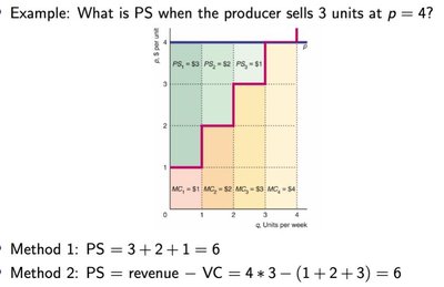
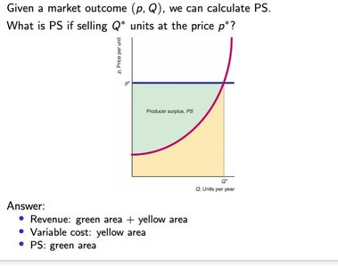
Producer Surplus (PS)

Producer surplus is the gain from trade, calculated as revenue minus variable cost. It can be found using the MC curve:

• Method 1: Add up marginal gains unit by unit.

• Method 2: $PS = \text{Revenue} - VC$

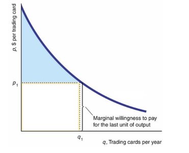
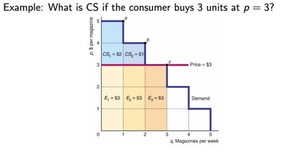
Consumer Surplus (CS)

Consumer surplus is the gain from trade, calculated as willingness to pay minus expenditure. The demand curve represents marginal willingness to pay.

• Method 1: Add up marginal gains unit by unit.

• Method 2: $CS = WTP - \text{Expenditure}$

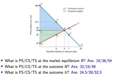
Total Surplus (TS)

Total surplus is the sum of producer and consumer surplus, representing social welfare:

• $TS = CS + PS$

• Market equilibrium maximizes total surplus.

Market Interventions

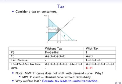
Tax

A tax on consumers or producers reduces the equilibrium quantity, leading to deadweight loss (DWL) and under-transaction.

	Without Tax	With Tax
PS	F+G+H+I	I
CS	A+B+C+D+E	A+B
Tax Revenue	-	C+D+F+G
TS	PS+CS+Tax Rev	PS+CS+Tax Rev
DWL	-	E+H

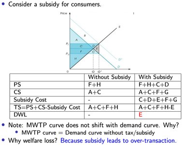
Subsidy

A subsidy increases the equilibrium quantity, leading to deadweight loss (DWL) and over-transaction.

	Without Subsidy	With Subsidy
PS	F+H	F+H+C+D
CS	A+C	A+C+F+G
Subsidy Cost	-	C+D+F+G
TS	PS+CS-Subsidy Cost	PS+CS-Subsidy Cost
DWL	-	E

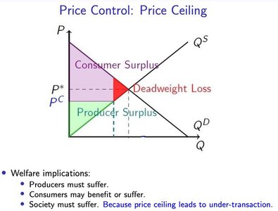
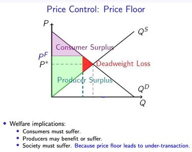
Price Controls

Price ceilings and floors cause deadweight loss by reducing the quantity traded below the competitive equilibrium.

• Price Ceiling: Leads to under-transaction; producers suffer, consumers may benefit or suffer, society suffers.

• Price Floor: Leads to under-transaction; consumers suffer, producers may benefit or suffer, society suffers.

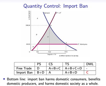
Import Ban and Tariff

Import bans and tariffs harm domestic consumers, benefit domestic producers, and reduce total surplus due to deadweight loss.

	Free Trade	Import Ban
PS	D	B+D
CS	A+B+C	A
TS	A+B+C+D	A+B+D
DWL	-	C

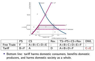
	Free Trade	Tariff
PS	F	B+F
CS	A+B+C+D+E	A
Rev.	-	D
TS	A+B+C+D+E+F	A+B+D+F
DWL	-	C+E

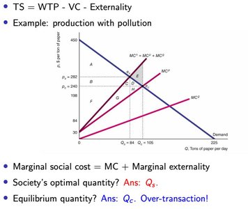
Externalities

Negative Externality

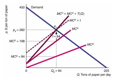
Negative externalities occur when a producer or consumer's actions directly harm others. Examples include pollution and manufacturing by-products. The equilibrium quantity is higher than the social optimum, leading to over-transaction.

• Marginal Social Cost: $MSC = MC + \text{Marginal Externality}$

• Remedies: Market for property rights (e.g., emissions trading), regulation (tax or quantity control).

Positive Externality

Positive externalities occur when a producer or consumer's actions directly benefit others. Examples include education and vaccination. The equilibrium quantity is lower than the social optimum, leading to under-transaction.

• Marginal Social Benefit: $MSB = MWTP + \text{Marginal Externality}$

• Remedies: Market for property rights, regulation (subsidy, government provision, mandate).

Additional info:

• All equations are provided in LaTeX format for clarity.

• Tables are recreated in HTML for comparison and classification purposes.

• Images are included only when directly relevant to the explanation of the adjacent paragraph.