Microeconomics Study Guide: Costs, Supply, Surplus, and Externalities

Firms and Production

Production Functions and Inputs

In microeconomics, firms transform inputs into outputs using technology. The production function describes this relationship mathematically.

• Production Function: $q = f(L, K)$, where q is output, L is labor, and K is capital.

• Isoquant Curve: A set of input bundles that produce the same output.

• Isoquant Map: Collection of isoquant curves for different output levels.

• Short Run: Some inputs (e.g., labor) are adjustable, others (e.g., capital) are fixed.

• Long Run: All inputs are adjustable.

Example: A factory may adjust labor daily but can only change machinery over years.

Costs

Short-Run Cost Functions

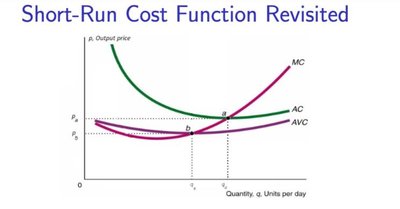
Short-run costs are divided into fixed and variable components. The cost functions help firms decide how much to produce.

• Fixed Cost (FC): Costs that do not change with output (e.g., rent).

• Variable Cost (VC): Costs that change with output (e.g., wages).

• Total Cost (TC): $TC(q) = VC(q) + FC$

• Marginal Cost (MC): $MC(q) = \Delta TC(q) / \Delta q = \Delta VC(q) / \Delta q$

• Average Cost (AC): $AC(q) = TC(q) / q$

• Average Variable Cost (AVC): $AVC(q) = VC(q) / q$

• Average Fixed Cost (AFC): $AFC(q) = FC / q$

Typical Properties: AC and AVC are U-shaped. MC intersects AC and AVC at their minimum points.

Long-Run Cost Functions

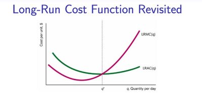
In the long run, all inputs are variable. The long-run average cost (LRAC) and long-run marginal cost (LRMC) are key concepts.

• Long-Run Cost Function: $LRC(q)$

• Long-Run Average Cost: $LRAC(q) = LRC(q) / q$

• Long-Run Marginal Cost: $LRMC(q)$

• LRAC is U-shaped: Decreases due to economies of scale, then increases due to diseconomies.

• Relationship:

  • When $q < q^*$: $LRMC < LRAC$

  • When $q = q^*$: $LRMC = LRAC$

  • When $q > q^*$: $LRMC > LRAC$

Supply Curves

Short-Run Individual Supply Curve

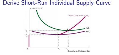
The short-run supply curve is the portion of the MC curve above AVC. Producers supply output where price is greater than or equal to AVC.

• Shut-down Price ($p_b$): If $p < p_b$, supply is zero.

• Break-even Price ($p_a$): If $p \geq p_a$, producer earns zero profit.

• Supply Decision: If $p \geq p_b$, produce where $MR = MC$.

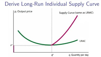
Long-Run Individual Supply Curve

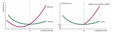
The long-run supply curve is the portion of the LRMC curve above LRAC. In the long run, producers can enter or exit freely.

• Long-Run Shut-down Price ($p^*$): If $p < p^*$, supply is zero.

• Break-even Price: $p^*$ is both shut-down and break-even price in the long run.

• Supply Decision: If $p \geq p^*$, produce where $MR = LRMC$.

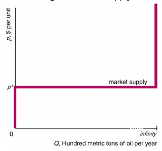
Market Supply Curve

The market supply curve aggregates individual supply curves. In the long run, the supply curve is horizontal at the break-even price if there are infinitely many identical producers.

• Short Run: Sum individual supply curves for given producers.

• Long Run: Entry and exit lead to a horizontal supply curve at $p^*$.

Economic Surplus

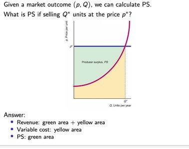
Producer Surplus (PS)

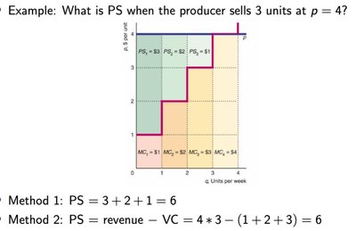
Producer surplus is the gain from trade for producers, calculated as revenue minus variable cost.

• PS Calculation: Two methods:

  • Sum marginal gains unit by unit.

  • PS = Revenue - VC

Consumer Surplus (CS)

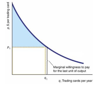
Consumer surplus is the gain from trade for consumers, calculated as willingness to pay minus expenditure.

• Marginal Willingness to Pay (MWTP): The demand curve represents MWTP.

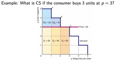
• CS Calculation: Two methods:

  • Sum marginal gains unit by unit.

  • CS = WTP - Expenditure

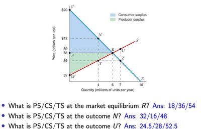
Total Surplus (TS)

Total surplus is the sum of producer and consumer surplus, representing social welfare.

• TS Formula: $TS = CS + PS = WTP - Expenditure + Revenue - VC$

• Market Equilibrium: Maximizes total surplus when MWTP = MC.

Market Interventions

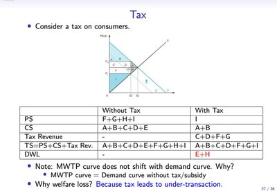
Tax

A tax reduces the quantity traded, leading to deadweight loss and lower total surplus.

• Tax Revenue: Collected by government.

• Deadweight Loss (DWL): Lost surplus due to under-transaction.

	Without Tax	With Tax
PS	F+G+H+I	I
CS	A+B+C+D+E	A+B
Tax Revenue	-	C+D+F+G
TS	PS+CS+Tax Rev	PS+CS+Tax Rev
DWL	-	E+H

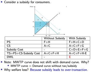
Subsidy

A subsidy increases the quantity traded, leading to deadweight loss from over-transaction.

• Subsidy Cost: Paid by government.

• Deadweight Loss (DWL): Lost surplus due to over-transaction.

	Without Subsidy	With Subsidy
PS	F+H	F+H+C+D
CS	A+C	A+C+F+G
Subsidy Cost	-	C+D+F+G
TS	PS+CS-Subsidy Cost	PS+CS-Subsidy Cost
DWL	-	E

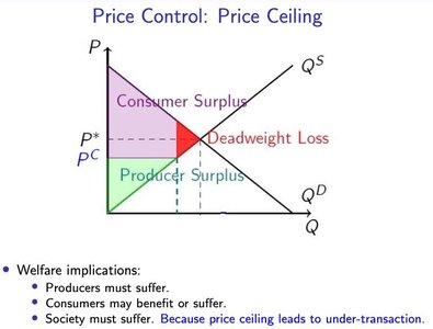
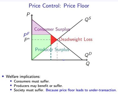
Price Controls

Price ceilings and floors cause deadweight loss by restricting market transactions.

• Price Ceiling: Maximum price allowed; leads to under-transaction.

• Price Floor: Minimum price allowed; also leads to under-transaction.

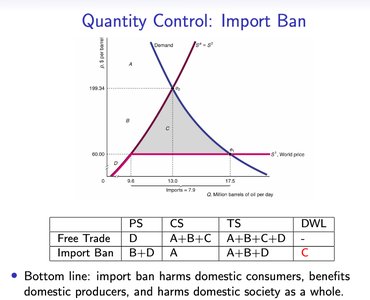
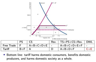
Import Ban and Tariff

Import bans and tariffs restrict trade, harming consumers and society overall, but benefiting domestic producers.

	Free Trade	Import Ban
PS	D	B+D
CS	A+B+C	A
TS	A+B+C+D	A+B+D
DWL	-	C

	Free Trade	Tariff
PS	F	B+F
CS	A+B+C+D+E	A
Rev.	-	D
TS	A+B+C+D+E+F	A+B+D+F
DWL	-	C+E

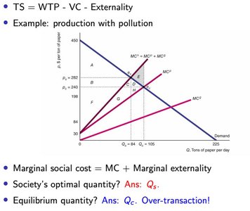
Externalities

Negative Externalities

Negative externalities occur when a producer or consumer's actions harm others. The market equilibrium typically results in over-transaction compared to the social optimum.

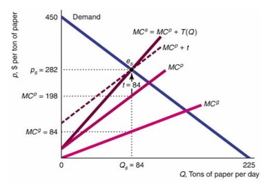
• Marginal Social Cost: $MSC = MC +$ Marginal externality

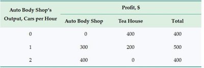
• Remedies: Property rights (market approach), taxes, or quantity controls (regulation approach).

Positive Externalities

Positive externalities occur when actions benefit others. The market equilibrium results in under-transaction compared to the social optimum.

• Marginal Social Benefit: $MSB = MWTP +$ Marginal externality

• Remedies: Property rights (market approach), subsidies, government provision, or mandates (regulation approach).

Summary Table: Key Formulas

• Average Product of Labor: $AP_L = Q / L$

• Profit: $\text{Profit} = \text{Revenue} - \text{Cost}$

• Short-Run Total Cost: $TC(q) = w \cdot L(q) + r \cdot K$

• Long-Run Average Cost: $LRAC(q) = LRC(q) / q$

• Producer Surplus: $PS = \text{Revenue} - VC$

• Consumer Surplus: $CS = WTP - \text{Expenditure}$

• Total Surplus: $TS = CS + PS$

Additional info: All diagrams and tables included are directly relevant to the explanation of the adjacent paragraphs, visually reinforcing key microeconomic concepts.