Oligopoly Models: Cournot, Bertrand, and Stackelberg Duopoly

Oligopoly Models

Introduction to Oligopoly

Oligopoly is a market structure characterized by a small number of firms whose decisions affect each other. The strategic interactions among firms can be modeled using game theory, with the most common models being Cournot, Bertrand, and Stackelberg duopolies.

• Cournot Duopoly: Firms simultaneously choose quantities to produce.

• Bertrand Duopoly: Firms simultaneously choose prices to post.

• Stackelberg Duopoly: Firms choose quantities sequentially, with one firm (the leader) moving first.

Cournot Duopoly Model

Definition and Equilibrium

In the Cournot model, each firm chooses its output level simultaneously, taking the other firm's output as given. The Nash equilibrium in this setting is called the Cournot equilibrium.

• Key Feature: Strategic interdependence in output decisions.

• Equilibrium Concept: Each firm's output is optimal given the output of the other firm.

Payoff Matrix Example

The following table shows the payoffs for two firms (Firm 1 and Firm 2) choosing among three output levels: Low (L), Medium (M), and High (H). Each cell contains the payoffs (Firm 1, Firm 2).

	L	M	H
L	112.5, 112.5	93.75, 125	56.25, 112.5
M	125, 93.75	100, 100	50, 75
H	112.5, 56.25	75, 50	0, 0

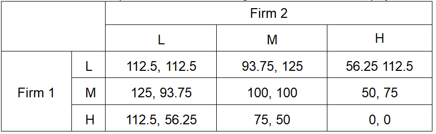
Example: The Cournot equilibrium occurs at (M, M), where both firms choose the medium output and each earns a payoff of 100.

Bertrand Duopoly Model

Definition and Equilibrium

In the Bertrand model, firms simultaneously choose prices. The Nash equilibrium in this setting is called the Bertrand equilibrium. Typically, if products are identical and marginal costs are constant, the equilibrium price equals marginal cost, resulting in zero economic profit for both firms.

• Key Feature: Price competition can drive prices down to marginal cost.

• Equilibrium Concept: Each firm's price is optimal given the price of the other firm.

Stackelberg Duopoly Model

Definition and Equilibrium

The Stackelberg model introduces sequential decision-making. The leader firm chooses its output first, and the follower observes this choice and then selects its own output. The equilibrium is called the Stackelberg equilibrium and is found using backward induction.

• Key Feature: First-mover advantage for the leader.

• Equilibrium Concept: Subgame perfect Nash equilibrium (SPNE).

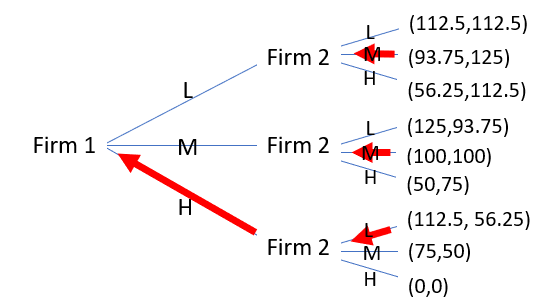
Game Tree Representation

The following diagram illustrates the sequential nature of the Stackelberg game, where Firm 1 moves first and Firm 2 responds optimally to each possible action by Firm 1. The red arrows indicate the optimal choices at each stage.

Solving the Stackelberg Equilibrium: Analytical Example

Consider a market with demand function $Q(p) = 1000 - 2p$, and cost functions $C_1(q_1) = 200q_1$ and $C_2(q_2) = 200q_2$. Firm 1 is the leader, and Firm 2 is the follower.

1. Step 1: Derive the Inverse Demand Function $Q = 1000 - 2p \implies p = 500 - 0.5Q$, where $Q = q_1 + q_2$.

2. Step 2: Follower's (Firm 2's) Problem

   • Revenue: $R_2 = (500 - 0.5q_1 - 0.5q_2)q_2 = 500q_2 - 0.5q_1q_2 - 0.5q_2^2$

   • Marginal Revenue: $MR_2 = 500 - 0.5q_1 - q_2$

   • Marginal Cost: $MC_2 = 200$

   • Set $MR_2 = MC_2$: $500 - 0.5q_1 - q_2 = 200 \implies q_2 = 300 - 0.5q_1$ (Firm 2's reaction function)

3. Step 3: Leader's (Firm 1's) Problem

   • Total output: $Q = q_1 + q_2 = q_1 + (300 - 0.5q_1) = 300 + 0.5q_1$

   • Price: $p = 500 - 0.5Q = 500 - 0.5(300 + 0.5q_1) = 350 - 0.25q_1$

   • Revenue: $R_1 = (350 - 0.25q_1)q_1 = 350q_1 - 0.25q_1^2$

   • Marginal Revenue: $MR_1 = 350 - 0.5q_1$

   • Marginal Cost: $MC_1 = 200$

   • Set $MR_1 = MC_1$: $350 - 0.5q_1 = 200 \implies q_1 = 300$

   • Substitute $q_1$ into follower's reaction: $q_2 = 300 - 0.5 \times 300 = 150$

4. Step 4: Equilibrium Outcomes

   • Firm 1 output: 300

   • Firm 2 output: 150

   • Total output: 450

   • Equilibrium price: $p = 500 - 0.5 \times 450 = 275$

   • Profit for Firm 1: $275 \times 300 - 200 \times 300 = 22500$

   • Profit for Firm 2: $275 \times 150 - 200 \times 150 = 11250$

Conclusion: The leader (Firm 1) enjoys a first-mover advantage, producing more and earning higher profit than the follower.

Graphical Comparison: Cournot vs. Stackelberg Equilibrium

In the Cournot equilibrium, both firms produce 200 units each. In the Stackelberg equilibrium, the leader produces 300 units and the follower produces 150 units. The reaction functions for both firms are:

• Firm 1: $q_1(q_2) = 300 - 0.5q_2$

• Firm 2: $q_2(q_1) = 300 - 0.5q_1$

Cournot Equilibrium: $(q_1, q_2) = (200, 200)$ Stackelberg Equilibrium: $(q_1, q_2) = (300, 150)$

Does the Leader Always Have an Advantage?

Not necessarily. If the leader has a higher marginal cost, the first-mover advantage can be offset or even reversed. For example, if $MC_1 = 250$ and $MC_2 = 200$, both firms produce 200 units, and the leader earns less profit than the follower.

• Key Insight: The first-mover advantage depends on cost structures as well as timing.

Summary Table: Cournot and Stackelberg Equilibria

Model	Firm 1 Output	Firm 2 Output	Price	Profit 1	Profit 2
Cournot	200	200	300	20000	20000
Stackelberg (MC=200)	300	150	275	22500	11250
Stackelberg (MC1=250, MC2=200)	200	200	300	<20000	>20000

Additional info: Table values for profit in the last row are inferred based on the discussion that the leader earns less than the follower when MC1 > MC2.