Producers in the Short Run: Production, Costs, and Profit in Microeconomics

Producers in the Short Run

Introduction

This chapter explores the behavior of firms in the short run, focusing on how they organize, finance, and make production decisions. It also examines the relationships among production, costs, and profits, providing the foundation for understanding the supply curve in microeconomics.

7.1 What Are Firms?

Forms of Business Organization

• Single Proprietorship: Owned and managed by one individual, who is personally liable for all debts (e.g., tradespeople).

• Ordinary Partnership: Two or more partners share responsibility and liability (e.g., start-ups).

• Limited Partnership: General partners manage and are liable; limited partners invest but have limited liability (e.g., law firms).

• Corporation: Legal entity separate from owners; liability is limited to investment. Private corporations' shares are not publicly traded; public corporations' shares are.

• State-Owned Enterprise (Crown Corporation): Government-owned, managed by a state-appointed board (e.g., ViaRail, Canada Post).

• Non-Profit Organization: Profits are reinvested; not distributed to individuals (e.g., YMCA).

Multinational Enterprises (MNEs): Firms operating in multiple countries, common among large corporations.

Not all production occurs within firms; government agencies also provide goods and services, typically funded by taxes.

Financing of Firms

• Financial Capital: Funds raised for business operations, distinct from physical capital (assets like machinery).

• Equity: Funds from owners/shareholders; profits may be paid as dividends or retained for investment.

• Debt: Borrowed funds from creditors, repaid with interest. Debt instruments include loans and bonds.

Goals of Firms

• Firms are generally assumed to be profit-maximizers and act as single, consistent decision-making units.

• There is ongoing debate about balancing profit maximization with social responsibility (e.g., environmental concerns, ethical practices).

7.2 Production, Costs, and Profits

Production and Inputs

• Production uses four types of inputs:

  1. Intermediate products (outputs from other firms, e.g., steel)

  2. Natural resources (e.g., land)

  3. Labour services

  4. Physical capital (e.g., machinery)

• Production Function: Describes the maximum output (Q) from given inputs of labour (L) and capital (K): $Q = f(L, K)$

• Production is a flow concept (output per period of time).

Costs and Profits

• Explicit Costs: Actual monetary payments (e.g., wages, rent, materials, depreciation).

• Implicit Costs: Opportunity costs of using resources owned by the firm (e.g., owner's time, capital).

• Accounting Profit: $\text{Accounting Profit} = \text{Revenues} - \text{Explicit Costs}$

• Economic Profit: $\text{Economic Profit} = \text{Revenues} - (\text{Explicit Costs} + \text{Implicit Costs})$ or $\text{Economic Profit} = \text{Accounting Profit} - \text{Implicit Costs}$

• Negative economic profit is called an economic loss.

Opportunity Cost of Time and Capital

• Owner's time: The difference between what the owner pays themselves and what they could earn elsewhere is an implicit cost.

• Owner's capital: The opportunity cost includes the risk-free rate (e.g., government bonds) and a risk premium.

Table: Accounting vs. Economic Profit Example

	Accounting Profit	Economic Profit
Total Revenues	$2000	$2000
Total Explicit Costs	$1160	$1160
Accounting Profit	$840	-
Total Implicit Costs	-	$265
Economic Profit	-	$575

Additional info: This table illustrates the calculation of both accounting and economic profit for a hypothetical firm.

Profits and Resource Allocation

• Resources flow to industries with the highest economic profits.

• Zero economic profit means no incentive for resources to move.

• Economic profits and losses signal where resources are most valued.

7.3 Production in the Short Run

Short-Run Production Concepts

• Total Product (TP): Total output produced with a given amount of input.

• Average Product (AP): Output per unit of variable input (usually labour): $AP = \frac{TP}{L}$

• Marginal Product (MP): Additional output from one more unit of variable input: $MP = \frac{\Delta TP}{\Delta L}$

Figure: The table and graphs show how total, average, and marginal product change as labour input increases. The point of diminishing marginal productivity is where MP reaches its maximum and begins to decline.

Law of Diminishing Marginal Returns

• If increasing amounts of a variable factor are applied to a fixed factor, the marginal product of the variable factor will eventually decline.

• Examples: Additional sets in a workout, more pollution filters, or more stocks in a portfolio all show diminishing returns at some point.

Average-Marginal Relationship

• When MP > AP, AP rises; when MP < AP, AP falls.

• MP curve intersects AP curve at AP's maximum point.

7.4 Firms’ Costs in the Short Run

Types of Short-Run Costs

• Total Cost (TC): $TC = TFC + TVC$

• Total Fixed Cost (TFC): Costs that do not vary with output (e.g., rent).

• Total Variable Cost (TVC): Costs that vary with output (e.g., labour, materials).

• Average Total Cost (ATC): $ATC = \frac{TC}{Q}$

• Average Fixed Cost (AFC): $AFC = \frac{TFC}{Q}$

• Average Variable Cost (AVC): $AVC = \frac{TVC}{Q}$

• Marginal Cost (MC): $MC = \frac{\Delta TC}{\Delta Q}$

Table: Short-Run Costs Example

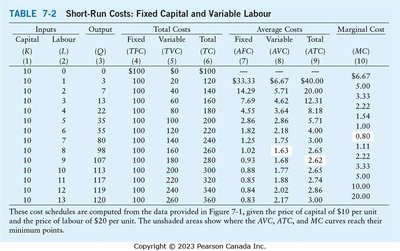
This table shows how costs are calculated for different levels of output, given fixed and variable inputs and their prices.

Short-Run Cost Curves

• TFC is constant; TC and TVC rise with output.

• AFC declines as output increases (spreading overhead).

• ATC and AVC are U-shaped due to the law of diminishing returns.

• MC curve intersects AVC and ATC at their minimum points.

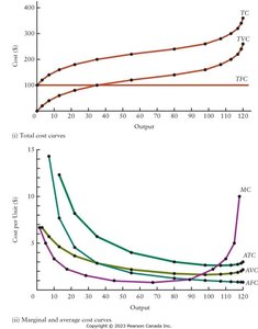
These figures illustrate the typical shapes of cost curves in the short run, showing the relationships among TC, TVC, TFC, ATC, AVC, AFC, and MC.

Why U-Shaped Cost Curves?

• AP and MP curves are hill-shaped; AVC and MC are U-shaped.

• When AP rises, AVC falls; when AP falls, AVC rises. Minimum AVC occurs at maximum AP.

• When MP rises, MC falls; when MP falls, MC rises. Minimum MC occurs at maximum MP.

• ATC is the sum of AFC (declining) and AVC (U-shaped); its minimum occurs after AVC's minimum.

Capacity

• Capacity: Output level at minimum short-run ATC.

• Producing below capacity means excess capacity.

Shifts in Short-Run Cost Curves

• Increase in variable factor price shifts AVC, ATC, and MC upward.

• Increase in fixed factor price shifts AFC and ATC upward; MC unchanged.

• Increasing fixed factors can lower AVC and MC by increasing productivity, but raises AFC.

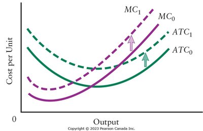
This figure shows how cost curves shift when input prices change.

Special Case: Digital Products

• Digital goods often have high fixed costs but near-zero marginal costs (e.g., software, video games).

• Law of diminishing returns may not apply; MC and AVC are constant and low, ATC declines as output increases.

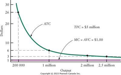
In digital industries, cost curves can look very different from traditional manufacturing due to negligible marginal costs.