Step-by-Step Microeconomics Exam Study Guide

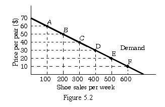
Q1. Refer to Figure 5.2. Using the initial-value method, the value of the price elasticity of demand from Point A to Point B can be described as:

Background

Topic: Price Elasticity of Demand

This question tests your understanding of how to calculate and interpret the price elasticity of demand using the initial-value method, which measures the responsiveness of quantity demanded to a change in price.

Key Terms and Formulas

• Price Elasticity of Demand ($E_d$): Measures how much quantity demanded changes in response to a price change.

• Initial-Value Method Formula:

$E_d = \frac{\%\,\text{change in quantity demanded}}{\%\,\text{change in price}}$

$\%\,\text{change in quantity demanded} = \frac{Q_2 - Q_1}{Q_1}$

$\%\,\text{change in price} = \frac{P_2 - P_1}{P_1}$

Step-by-Step Guidance

1. Identify the coordinates for Points A and B from Figure 5.2 (price and quantity values).

2. Calculate the percentage change in quantity demanded using the initial value (from A to B).

3. Calculate the percentage change in price using the initial value (from A to B).

4. Set up the elasticity formula using your calculated percentage changes.

5. Interpret the elasticity value: If $E_d > 1$, demand is elastic; if $E_d = 1$, unit elastic; if $E_d < 1$, inelastic.

Try solving on your own before revealing the answer!

Final Answer: Elastic (D)

Using the initial-value method, the elasticity from A to B is greater than 1, indicating elastic demand.

This means consumers are highly responsive to price changes in this range.

Q2. Refer to Figure 5.2. Using the initial-value method, the value of the price elasticity of demand from Point E to Point F can be described as:

Background

Topic: Price Elasticity of Demand (Lower Portion of Demand Curve)

This question tests your ability to calculate price elasticity at a different segment of the demand curve, where elasticity often changes.

Key Terms and Formulas

• Price Elasticity of Demand ($E_d$): Same formula as above.

• Interpretation: Lower segments of the demand curve tend to be less elastic.

$E_d = \frac{\%\,\text{change in quantity demanded}}{\%\,\text{change in price}}$

Step-by-Step Guidance

1. Find the price and quantity values for Points E and F from Figure 5.2.

2. Calculate the percentage change in quantity demanded using the initial value (E).

3. Calculate the percentage change in price using the initial value (E).

4. Set up the elasticity formula with your calculated values.

5. Compare the elasticity value to 1 to determine if demand is elastic, unit elastic, or inelastic.

Try solving on your own before revealing the answer!

Final Answer: Inelastic (D)

The elasticity from E to F is less than 1, indicating inelastic demand. Consumers are less responsive to price changes in this range.

Q3. When the price of charcoal grills increases, total revenue increases for charcoal grill retailers. From this information, we can conclude that:

Background

Topic: Relationship Between Price Elasticity and Total Revenue

This question tests your understanding of how price elasticity affects total revenue when prices change.

Key Terms and Formulas

• Total Revenue ($TR$): $TR = P \times Q$

• Elasticity and Revenue: If demand is inelastic, increasing price increases total revenue.

Step-by-Step Guidance

1. Recall the definition of inelastic demand: $E_d < 1$.

2. Understand that with inelastic demand, a price increase leads to a smaller decrease in quantity demanded.

3. Apply the total revenue formula to see how $TR$ changes when price increases and demand is inelastic.

4. Use this reasoning to determine which option best describes the demand for charcoal grills.

Try solving on your own before revealing the answer!

Final Answer: The demand for charcoal grills is inelastic (C)

Since total revenue increases when price increases, demand must be inelastic.

Q4. Assume that Crystal's demand for soup remains constant, but the price of soup increases. Crystal's consumer surplus:

Background

Topic: Consumer Surplus

This question tests your understanding of how changes in price affect consumer surplus, which is the difference between what a consumer is willing to pay and what they actually pay.

Key Terms and Formulas

• Consumer Surplus: Area between the demand curve and the price line, up to the quantity purchased.

• Price Increase: Reduces consumer surplus.

Step-by-Step Guidance

1. Recall the definition of consumer surplus.

2. Visualize the effect of a price increase on the area under the demand curve above the new price.

3. Reason through whether the surplus increases, decreases, or stays the same.

4. Consider the options and select the one that matches your reasoning.

Try solving on your own before revealing the answer!

Final Answer: Consumer surplus decreases (B)

When price increases, the area representing consumer surplus shrinks.

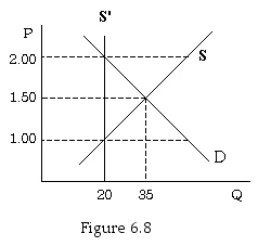
Q5. Refer to Figure 6.8. If the government limits taxicab services to 20 per day, the price per mile traveled will be:

Background

Topic: Price Controls and Market Equilibrium

This question tests your ability to interpret supply and demand graphs and understand the effects of quantity restrictions.

Key Terms and Formulas

• Market Equilibrium: Where supply and demand intersect.

• Quantity Restriction: Government-imposed limit on quantity.

Step-by-Step Guidance

1. Locate the quantity restriction (20 rides per day) on the horizontal axis of Figure 6.8.

2. Find the corresponding price where the vertical line at 20 intersects the supply curve.

3. Compare this price to the equilibrium price (where supply and demand intersect).

4. Identify the price per mile at the restricted quantity.

Try solving on your own before revealing the answer!

Final Answer: $2.00 (C)

At the restricted quantity, the price per mile is $2.00, as shown by the intersection with the supply curve.

Q6. Laura makes hand-made jewelry and she would be willing to sell pairs of earrings for $50. If Laura sells each pair of earrings for $65, her producer surplus per pair of earrings sold would be equal to:

Background

Topic: Producer Surplus

This question tests your understanding of producer surplus, which is the difference between the price received and the minimum price the producer is willing to accept.

Key Terms and Formulas

• Producer Surplus: $\text{Producer Surplus} = \text{Price Received} - \text{Willingness to Sell}$

Step-by-Step Guidance

1. Identify the price Laura receives ($65) and her minimum acceptable price ($50).

2. Set up the producer surplus formula.

3. Subtract the minimum price from the price received to find the surplus per pair.

Try solving on your own before revealing the answer!

Final Answer: $15 (D)

Producer surplus is $65 - $50 = $15 per pair.

Q7. The budget line shows:

Background

Topic: Budget Constraint

This question tests your understanding of the budget line, which represents all combinations of two goods a consumer can purchase given their income and prices.

Key Terms and Formulas

• Budget Line: $P_x X + P_y Y = I$

• Where $P_x$ and $P_y$ are prices, $X$ and $Y$ are quantities, and $I$ is income.

Step-by-Step Guidance

1. Recall the definition of the budget line.

2. Understand that it shows all possible combinations of two goods that exhaust the consumer's income.

3. Compare the options to see which best matches this definition.

Try solving on your own before revealing the answer!

Final Answer: The different combinations of two goods that a consumer can buy (B)

The budget line shows all combinations of two goods a consumer can afford.

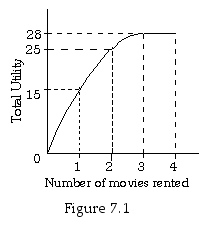
Q8. Refer to Figure 7.1. The marginal utility of the second movie rental is:

Background

Topic: Marginal Utility

This question tests your ability to calculate marginal utility, which is the additional satisfaction from consuming one more unit of a good.

Key Terms and Formulas

• Marginal Utility: $MU = TU_2 - TU_1$

• $TU$ = Total Utility

Step-by-Step Guidance

1. Find the total utility for renting one and two movies from Figure 7.1.

2. Subtract the total utility of one movie from the total utility of two movies to find the marginal utility of the second rental.

3. Compare your result to the answer choices.

Try solving on your own before revealing the answer!

Final Answer: 10 (A)

Marginal utility is the increase in total utility from renting the second movie.

Q9. When income increases:

Background

Topic: Budget Constraint Shifts

This question tests your understanding of how changes in income affect the budget constraint.

Key Terms and Formulas

• Budget Constraint: $P_x X + P_y Y = I$

• Income Increase: Shifts the budget line outward (parallel shift).

Step-by-Step Guidance

1. Recall what happens to the budget line when income increases (holding prices constant).

2. Visualize the shift: the consumer can afford more of both goods.

3. Determine which option best describes this effect.

Try solving on your own before revealing the answer!

Final Answer: The budget constraint will shift out (C)

Increasing income shifts the budget line outward, allowing more combinations of goods.

Q10. You are the owner and only employee of a company that repairs computers. Last year, you earned total revenues of $75,000. Your costs for equipment, rent, and supplies were $10,000. To start this business you quit a job at a computer software firm that paid $40,000 a year. Last year, your economic profits were:

Background

Topic: Economic Profit vs. Accounting Profit

This question tests your understanding of economic profit, which includes opportunity costs.

Key Terms and Formulas

• Economic Profit: $\text{Economic Profit} = \text{Total Revenue} - (\text{Explicit Costs} + \text{Implicit Costs})$

• Explicit Costs: Out-of-pocket expenses ($10,000)

• Implicit Costs: Opportunity cost of foregone salary ($40,000)

Step-by-Step Guidance

1. Identify total revenue ($75,000), explicit costs ($10,000), and implicit costs ($40,000).

2. Set up the economic profit formula.

3. Subtract explicit and implicit costs from total revenue.

Try solving on your own before revealing the answer!

Final Answer: $25,000 (D)

Economic profit is $75,000 - $10,000 - $40,000 = $25,000.

Q11. A fixed cost can be thought of as:

Background

Topic: Fixed vs. Variable Costs

This question tests your understanding of fixed costs, which do not change with output.

Key Terms and Formulas

• Fixed Cost: Cost that must be paid even if output equals zero.

• Variable Cost: Changes with output.

Step-by-Step Guidance

1. Recall the definition of fixed cost.

2. Compare fixed cost to variable cost.

3. Identify which option best matches the definition.

Try solving on your own before revealing the answer!

Final Answer: A cost that must be paid even if output equals zero (C)

Fixed costs are incurred regardless of production level.

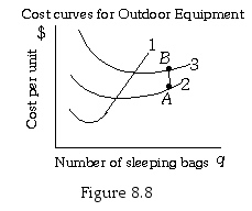
Q12. Refer to Figure 8.8. Curve 1 is Outdoor Equipment's:

Background

Topic: Cost Curves in Production

This question tests your ability to identify different cost curves in a firm's production graph.

Key Terms and Formulas

• Marginal Cost (MC): The cost of producing one more unit.

• Average Variable Cost (AVC), Average Total Cost (ATC), Average Fixed Cost (AFC): Other cost curves.

Step-by-Step Guidance

1. Examine the shape and position of Curve 1 in Figure 8.8.

2. Recall that the marginal cost curve typically intersects the average cost curves at their minimum points.

3. Compare Curve 1 to the typical marginal cost curve.

4. Identify which cost curve Curve 1 represents.

Try solving on your own before revealing the answer!

Final Answer: Marginal cost curve (A)

Curve 1 is the marginal cost curve, which shows the cost of producing each additional unit.