 Back
BackTechnology, Production, and Costs: Microeconomics Chapter 11 Study Guide
Study Guide - Smart Notes
 Tailored notes based on your materials, expanded with key definitions, examples, and context.
Technology, Production, and Costs
11.1 Technology: An Economic Definition
Technology in economics refers to the processes a firm uses to turn inputs into outputs of goods and services. Technological change occurs when a firm improves or worsens its ability to produce a given level of output with a given quantity of inputs.
Technology: The set of methods and processes used to transform inputs (such as labor, capital, and natural resources) into outputs.
Technological change: A positive or negative shift in a firm’s production capabilities, often due to innovation or new methods.
Example: The introduction of AI chatbots like ChatGPT is a technological change that can substitute capital for labor, increasing productivity for some workers while reducing jobs for others.
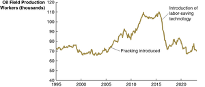
Apply the Concept: Oil Roughnecks Encounter Robots and Drones
Fracking technology increased demand for oil workers, but falling oil prices led firms to adopt labor-saving technologies such as robots and drones, reducing the workforce.
Positive technological change: Fracking increased productivity and demand for labor.
Labor-saving technology: Robots and drones reduced the number of workers needed by about 40,000.
11.2 The Short Run and the Long Run in Economics
Economists distinguish between the short run and the long run based on the flexibility of inputs. In the short run, at least one input is fixed; in the long run, all inputs can be varied.
Short run: Period during which at least one input (e.g., factory size) is fixed.
Long run: Period long enough for all inputs to be variable, allowing firms to adopt new technology or change plant size.
Example: A firm with a long-term lease on a factory cannot change its size in the short run but can do so in the long run.
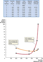
Fixed, Variable, and Total Costs
Variable costs: Costs that change as output changes (e.g., wages for workers).
Fixed costs: Costs that remain constant regardless of output (e.g., rent for factory).
Total cost: The sum of all costs incurred in production.
In the long run, all costs are variable.
Implicit Costs Versus Explicit Costs
Explicit cost: Direct monetary expenditure (e.g., wages, rent).
Implicit cost: Nonmonetary opportunity cost (e.g., foregone salary, interest on invested capital).
Example: Jill Johnson’s foregone salary and economic depreciation are implicit costs of running her pizza store.
11.3 The Marginal Product of Labor and the Average Product of Labor
The marginal product of labor measures the additional output from hiring one more worker, while the average product of labor is the total output divided by the number of workers. Specialization and division of labor can increase productivity, but eventually diminishing returns set in.
Marginal product of labor: The extra output produced by adding one more worker.
Average product of labor: Total output divided by the number of workers.
Law of diminishing returns: Adding more of a variable input to a fixed input eventually causes the marginal product to decline.
Example: Adam Smith’s pin factory: Division of labor increased output per worker dramatically.
Graphical Illustration
As more workers are hired, total output increases but at a decreasing rate, illustrating diminishing returns.
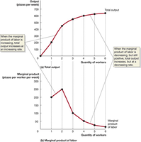
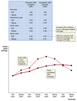
Average and Marginal Product of Labor
If the marginal product of the next worker is higher than the average, the average rises; if lower, the average falls.
Example: GPA analogy: Semester GPA above cumulative GPA raises the average; below lowers it.
11.4 The Relationship Between Short-Run Production and Short-Run Cost
Marginal cost is the change in total cost from producing one more unit. Average total cost is total cost divided by output. The relationship between these costs is central to understanding firm behavior.
Marginal cost (MC):
Average total cost (ATC):
When MC is below ATC, ATC falls; when MC is above ATC, ATC rises.
The ATC curve is typically U-shaped due to diminishing returns.
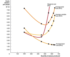
11.5 Graphing Cost Curves
Cost curves illustrate the relationships among average total cost, average variable cost, average fixed cost, and marginal cost. These curves help firms understand how costs change with output.
Average fixed cost (AFC):
Average variable cost (AVC):
Average total cost (ATC):
MC cuts ATC and AVC at their minimum points.
AFC declines as output increases, causing ATC and AVC to converge.
11.6 Costs in the Long Run
In the long run, all inputs are variable and firms use the long-run average cost curve for planning. This curve shows the lowest possible cost for producing each output level when no inputs are fixed.
Economies of scale: Long-run average costs fall as output increases.
Minimum efficient scale: The output level at which economies of scale are exhausted.
Constant returns to scale: Long-run average cost remains unchanged as output increases.
Diseconomies of scale: Long-run average costs rise as output increases, often due to management difficulties or less efficient use of resources.
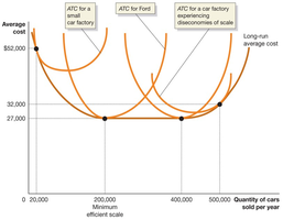
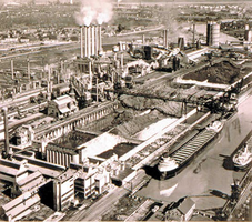
Apply the Concept: Diseconomies of Scale at Ford Motor Company
Ford’s River Rouge complex was so large that it became inefficient, illustrating diseconomies of scale. The disconnect between workers and management led to losses despite the potential for economies of scale.
Summary Table: Types of Costs
Type of Cost | Definition | Formula |
|---|---|---|
Fixed Cost (FC) | Cost that does not change with output | --- |
Variable Cost (VC) | Cost that changes with output | --- |
Total Cost (TC) | Sum of all costs | |
Average Fixed Cost (AFC) | Fixed cost per unit | |
Average Variable Cost (AVC) | Variable cost per unit | |
Average Total Cost (ATC) | Total cost per unit | |
Marginal Cost (MC) | Cost of one more unit |
Additional info: This guide expands on brief points with academic context, definitions, and examples to ensure completeness and clarity for exam preparation.
