Chapter 11

Technology, Production, and Costs

Technological Change and Production Costs

Technological advancements play a crucial role in reducing production costs and increasing output. In economics, technology refers to the process a firm uses to transform inputs into outputs, not just new inventions.

• Technology: The process a firm uses to convert inputs (workers, machines, natural resources, entrepreneurial skill) into outputs.

• Positive Technological Change: Improvements that allow firms to produce more with the same resources or the same output with fewer resources, shifting the supply curve right and expanding the production possibilities frontier (PPF).

• Negative Technological Change: Events that reduce a firm's ability to produce output with given inputs (e.g., hiring less skilled workers, natural disasters).

• Just-In-Time Inventory (JIT): A system that minimizes inventory levels, reducing opportunity costs and increasing efficiency, but may risk stock-outs.

Short Run vs. Long Run in Production

Firms analyze production and costs differently in the short run and long run. The distinction is based on the flexibility of inputs.

• Short Run (SR): At least one input is fixed; some costs are fixed, others are variable.

• Long Run (LR): All inputs are variable; firms can adjust technology, capital, and plant size.

• Formulas:

  • $\text{TC} = \text{FC} + \text{VC}$

  • $\text{ATC} = \text{AFC} + \text{AVC}$

  • In LR: $\text{TC} = \text{VC}$ and $\text{ATC} = \text{AVC}$

Types of Costs

Understanding cost structures is essential for economic analysis. Costs are categorized as variable or fixed, and as explicit or implicit.

• Variable Costs (VC): Costs that change with output (e.g., raw materials, hourly labor).

• Fixed Costs (FC): Costs that remain constant regardless of output (e.g., lease payments, insurance).

• Explicit Costs: Direct monetary expenditures (e.g., wages, rent).

• Implicit Costs: Opportunity costs (e.g., foregone salary, interest on invested capital).

• Economic Depreciation: The reduction in value of assets over time due to wear and tear or obsolescence.

• Economic Cost: $\text{Economic Cost} = \text{Explicit Costs} + \text{Implicit Costs}$

Cost Classification Table

This table summarizes the classification of costs by their nature:

Cost Type	Explicit/Implicit	Variable/Fixed
Labor (hourly)	Explicit	Variable
Raw materials	Explicit	Variable
Lease payments	Explicit	Fixed
Foregone salary	Implicit	Fixed
Interest on invested capital	Implicit	Variable/Fixed
Economic depreciation	Implicit	Variable/Fixed

Production Function

The production function describes the relationship between inputs and maximum output.

• Production Function: Relationship between inputs employed and maximum output produced.

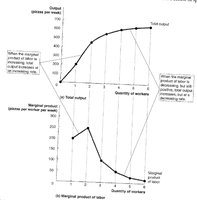
• Marginal Product of Labor (MPL): Additional output from hiring one more worker.

  • $\text{MPL} = \frac{\text{Change in Output}}{\text{Change in Labor}}$

• Division of Labor: Assigning specific tasks to workers increases efficiency.

• Specialization: Workers focus on fewer tasks to become more efficient.

• Law of Diminishing Returns: Adding more of a variable input to a fixed input eventually decreases the marginal product.

Short Run Cost Curves

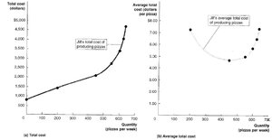
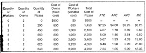
Cost curves illustrate how costs change with output in the short run. The total cost (TC) curve and average total cost (ATC) curve are key tools.

• Total Cost Curve (TC): Shows total cost for each output level; starts at the fixed cost.

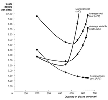
• Average Total Cost Curve (ATC): U-shaped due to division of labor, specialization, and diminishing returns.

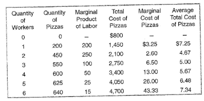
• Marginal Cost (MC): Change in total cost from producing one more unit.

  • $\text{MC} = \frac{\text{Change in TC}}{\text{Change in Q}}$

• Relationship: When MPL rises, MC falls; when MPL falls, MC rises.

Average and Marginal Cost Relationships

Understanding the relationship between marginal cost and average cost is essential for optimal production decisions.

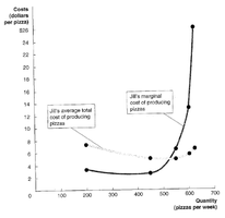
• MC curve intersects ATC and AVC curves at their minimum points.

• When MC < ATC/AVC, ATC/AVC decreases; when MC > ATC/AVC, ATC/AVC increases.

• AFC decreases as output increases, never rises.

• Difference between ATC and AVC decreases as output increases.

Long Run Average Cost (LRAC) and Economies of Scale

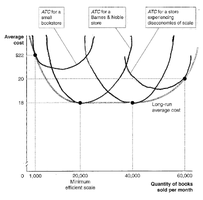
In the long run, all costs are variable, and the LRAC curve shows the lowest possible cost for each output level.

• LRAC Curve: Shows minimum cost for producing each output level when all inputs are variable.

• Economies of Scale: LRAC falls as output increases due to factors like division of labor, quantity discounts, lower interest rates, specialization, and bargaining power.

• Minimum Efficient Scale: Output level where all economies of scale are exhausted.

• Constant Returns to Scale: LRAC remains unchanged as output increases.

• Diseconomies of Scale: LRAC rises as output increases, often due to coordination difficulties in large firms.

Isoquants and Isocost Lines: Optimal Input Combination

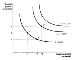
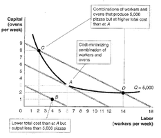
Firms use isoquants and isocost lines to determine the optimal mix of inputs for production.

• Isoquant: Curve showing all combinations of two inputs (e.g., labor and capital) that produce the same output.

• Isocost Line: Shows all combinations of two inputs with the same total cost.

• Marginal Rate of Technical Substitution (MRTS): Rate at which one input can be substituted for another while keeping output constant.

• Optimal Input Combination: Occurs where the isoquant is tangent to the isocost line.

  • $\frac{\text{MPL}}{\text{Price of Labor}} = \frac{\text{MPC}}{\text{Price of Capital}}$

Summary Table: Cost Concepts

Concept	Definition	Formula
Total Cost (TC)	Sum of all costs	$\text{TC} = \text{FC} + \text{VC}$
Average Total Cost (ATC)	Cost per unit	$\text{ATC} = \frac{\text{TC}}{Q}$
Average Fixed Cost (AFC)	Fixed cost per unit	$\text{AFC} = \frac{\text{FC}}{Q}$
Average Variable Cost (AVC)	Variable cost per unit	$\text{AVC} = \frac{\text{VC}}{Q}$
Marginal Cost (MC)	Cost of one more unit	$\text{MC} = \frac{\Delta \text{TC}}{\Delta Q}$
Marginal Product of Labor (MPL)	Output from one more worker	$\text{MPL} = \frac{\Delta \text{Output}}{\Delta \text{Labor}}$
LRAC	Lowest cost in long run	—
MRTS	Rate of input substitution	—

Additional info: Academic context and examples were added to clarify definitions, relationships, and applications for microeconomics students.