 Back
BackCh.11 Technology, Production, and Costs: Microeconomics Study Notes
Study Guide - Smart Notes
 Tailored notes based on your materials, expanded with key definitions, examples, and context.
Technology, Production, and Costs
Technology: An Economic Definition
Technology in economics refers to the processes a firm uses to turn inputs into outputs of goods and services. Technological change occurs when a firm improves or worsens its ability to produce a given level of output with a given quantity of inputs.
Technology: The set of processes used by firms to transform inputs (such as labor, capital, and natural resources) into outputs.
Technological Change: A positive or negative shift in a firm's production capabilities, often due to innovation or new methods.
Example: The adoption of artificial intelligence (AI) and automation, such as robots and drones in oil production, can increase productivity but may also reduce the demand for labor.

The Short Run and the Long Run in Economics
Economists distinguish between the short run and the long run based on the flexibility of input usage. In the short run, at least one input is fixed, while in the long run, all inputs can be varied.
Short Run: A period during which at least one input (e.g., capital) is fixed.
Long Run: A period long enough for all inputs to be variable; firms can adjust all factors of production.
Fixed Costs: Costs that do not change with the level of output (e.g., rent, machinery).
Variable Costs: Costs that change as output changes (e.g., labor, raw materials).
Total Cost: The sum of fixed and variable costs for a given level of output.
Example: In publishing, the cost of printing machines is fixed, while the cost of paper and labor varies with the number of books produced.

Implicit Costs Versus Explicit Costs
Economists consider both explicit and implicit costs when analyzing firm decisions. Explicit costs involve direct monetary payments, while implicit costs represent the opportunity costs of using resources owned by the firm.
Explicit Cost: A cost that involves a direct monetary payment (e.g., wages, rent).
Implicit Cost: The opportunity cost of using resources owned by the firm (e.g., foregone salary, interest income).
Example: If an entrepreneur quits a salaried job to start a business, the foregone salary is an implicit cost.
Production Functions and Short-Run Costs
The production function describes the relationship between the inputs employed by a firm and the maximum output it can produce. In the short run, some inputs are fixed, and others are variable.
Production Function: Shows the maximum output that can be produced with different combinations of inputs.
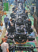
Example: Jill Johnson’s restaurant uses pizza ovens (fixed input) and workers (variable input) to produce pizzas.
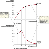
The Marginal Product of Labor and the Average Product of Labor
The marginal product of labor (MPL) is the additional output produced by hiring one more worker. The average product of labor (APL) is the total output divided by the number of workers. Specialization and division of labor can increase productivity, but eventually, diminishing returns set in.
Marginal Product of Labor (MPL): The change in output from hiring one additional worker.
Average Product of Labor (APL): Total output divided by the number of workers.
Law of Diminishing Returns: Adding more of a variable input to a fixed input will eventually cause the marginal product of the variable input to decline.
Example: In a pin factory, division of labor allowed for massive increases in productivity, as described by Adam Smith.

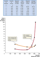
The Relationship Between Short-Run Production and Short-Run Cost
Marginal cost (MC) is the change in total cost from producing one more unit of output. The average total cost (ATC) is total cost divided by output. The MC curve typically intersects the ATC curve at its minimum point, creating a U-shaped ATC curve.
Marginal Cost (MC):
Average Total Cost (ATC):
Relationship: When MC is below ATC, ATC falls; when MC is above ATC, ATC rises.
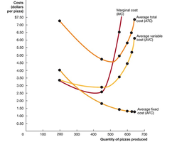
Graphing Cost Curves
Cost curves illustrate the relationships among average total cost, average variable cost, average fixed cost, and marginal cost. The ATC and AVC curves are U-shaped, and the MC curve intersects both at their minimum points.
Average Fixed Cost (AFC):
Average Variable Cost (AVC):
Relationship:
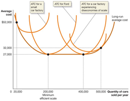
Costs in the Long Run
In the long run, all inputs are variable, and firms can adjust their scale of operation. The long-run average cost (LRAC) curve shows the lowest possible cost of producing each output level when all inputs can be varied.
Economies of Scale: LRAC decreases as output increases due to factors like specialization and bulk purchasing.
Minimum Efficient Scale: The lowest output level at which economies of scale are fully exploited.
Constant Returns to Scale: LRAC remains unchanged as output increases.
Diseconomies of Scale: LRAC increases as output increases, often due to management inefficiencies.
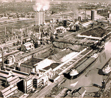
Example: Ford’s River Rouge complex became too large to manage efficiently, resulting in diseconomies of scale.
Appendix: Using Isoquants and Isocost Lines to Understand Production and Cost
Isoquants and isocost lines are tools used to analyze the cost-minimizing combination of inputs for a given level of output.
Isoquant: A curve showing all combinations of two inputs that yield the same output.
Isocost Line: A line showing all combinations of two inputs that cost the same total amount.
Marginal Rate of Technical Substitution (MRTS): The rate at which a firm can substitute one input for another while keeping output constant.
Cost Minimization: Achieved where the isoquant is tangent to the isocost line, i.e., where (the last dollar spent on each input yields the same marginal product).
Expansion Path: Shows the cost-minimizing input combinations as output increases.

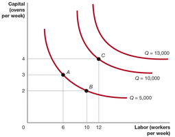

Additional info: Isoquants are analogous to indifference curves in consumer theory, while isocost lines are analogous to budget constraints. The tangency point represents the optimal input mix for cost minimization.
