Technology, Production, and Costs; The Markets for Labour and Other Factors of Production

Technology, Production, and Costs

Introduction to Firm Objectives and Profit Maximization

Firms are assumed to maximize profits, which is the difference between total revenue and total economic costs. Understanding how firms make decisions about input use, output levels, and product mix is central to microeconomic analysis.

• Profit (P): $P = TR - TC$

• Total Revenue (TR): $TR = P \times Q$

• Total Cost (TC): $TC = VC + FC$

Firms choose inputs and outputs to maximize profit, considering both revenues and costs.

Production Functions and Efficiency

The production function describes the maximum output that can be produced with a given set of inputs, reflecting the firm's technology. Inputs are also called factors of production. The production function, combined with input prices, determines the firm's cost structure.

• Production Function (Cobb-Douglas example): $Y = A L^a K^b$

• Marginal Product (MP): The additional output from using one more unit of an input, holding others fixed.

The Short Run and the Long Run

Economic analysis distinguishes between the short run (SR) and the long run (LR):

• Short Run (SR): At least one input is fixed.

• Long Run (LR): All inputs are variable; firms can adjust all factors, adopt new technology, and change plant size.

Types of Costs

Costs are categorized as fixed or variable, and as explicit or implicit:

• Fixed Costs (FC): Do not change with output (e.g., rent, equipment leases).

• Variable Costs (VC): Change with output (e.g., wages, materials).

• Explicit Costs: Actual monetary payments.

• Implicit Costs: Non-monetary opportunity costs (e.g., foregone salary).

Example Table: Explicit and Implicit Costs

Cost Item	Explicit Cost ($)	Implicit Cost ($)
Paper	20,000	-
Wages	48,000	-
Lease (machines)	10,000	-
Electricity	6,000	-
Lease (store)	24,000	-
Foregone salary	-	40,000
Foregone interest	-	3,000
Economic depreciation	-	10,000
Total	108,000	53,000

Additional info: Economic cost includes both explicit and implicit costs.

Short-Run Production and Cost Example

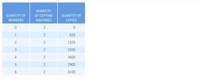
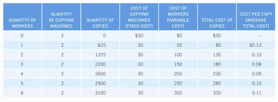
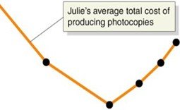
The following table shows how output and costs change as more workers are hired, holding capital fixed:

Marginal and Average Product of Labour

The marginal product of labour (MPL) is the additional output from hiring one more worker. The average product of labour (APL) is total output divided by the number of workers. The law of diminishing returns states that MPL eventually declines as more workers are added to a fixed amount of capital.

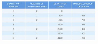
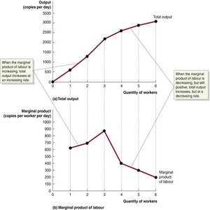
• MPL: $MPL = \frac{\Delta Q}{\Delta L}$

• APL: $APL = \frac{Q}{L}$

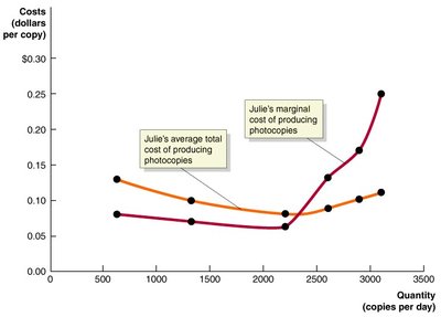
Cost Curves: Marginal, Average, and Total Costs

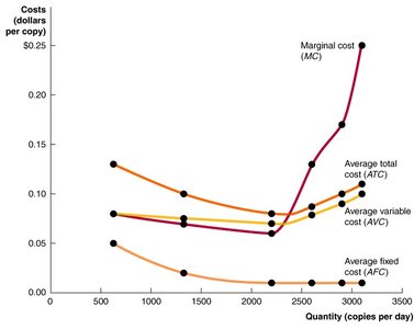
Cost curves are central to understanding firm behavior. Key relationships include:

• Marginal Cost (MC): $MC = \frac{\Delta TC}{\Delta Q}$

• Average Total Cost (ATC): $ATC = \frac{TC}{Q}$

• Average Fixed Cost (AFC): $AFC = \frac{FC}{Q}$

• Average Variable Cost (AVC): $AVC = \frac{VC}{Q}$

• ATC = AFC + AVC

The MC curve typically intersects the AVC and ATC curves at their minimum points. As output increases, AFC declines, and the gap between ATC and AVC narrows.

Long-Run Costs and Economies of Scale

In the long run, all inputs are variable. The long-run average cost curve (LRAC) shows the lowest possible cost of producing each output level when the firm can adjust all inputs. Key concepts:

• Economies of Scale: LRAC decreases as output increases.

• Constant Returns to Scale: LRAC remains unchanged as output increases.

• Diseconomies of Scale: LRAC increases as output increases.

• Minimum Efficient Scale (MES): The smallest output at which LRAC is minimized.

Cost Minimization and Input Choice

Firms minimize costs by choosing the optimal combination of inputs. The cost-minimizing rule is:

• $\frac{MPL}{w} = \frac{MPK}{r}$

Where w is the wage rate and r is the rental rate of capital. This can be illustrated with isoquants (curves showing combinations of inputs that yield the same output) and isocost lines (combinations of inputs that cost the same).

The Markets for Labour and Other Factors of Production

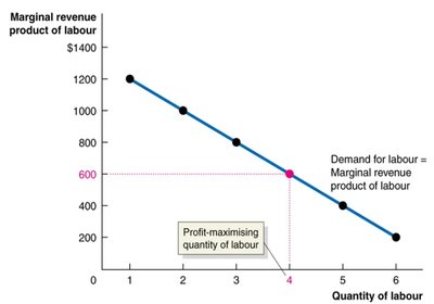
Labour Demand

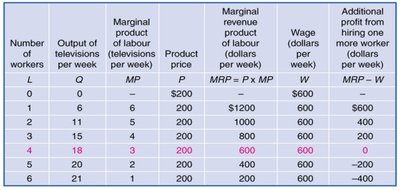
The demand for labour is derived from the demand for the goods and services produced. The marginal revenue product of labour (MRPL) is the additional revenue from hiring one more worker:

• If price is constant: $MRPL = MPL \times P$

• If price varies: $MRPL = \frac{dTR}{dL}$

The firm hires workers up to the point where $MRPL = W$ (wage rate).

Labour Supply

The labour supply curve shows the relationship between the wage rate and the quantity of labour supplied. It is typically upward-sloping, but may bend backward at high wage levels due to the income effect (preference for leisure increases as income rises).

Equilibrium in the Labour Market

Labour market equilibrium occurs where labour demand equals labour supply. Changes in demand or supply shift the equilibrium wage and employment level.

Explaining Wage Differences

Wage differences arise due to differences in productivity (MRPL), demand for specific skills, and supply of workers. For example, top athletes may earn more than university lecturers due to higher MRPL.

The Markets for Capital and Natural Resources

Capital (machines, buildings) and natural resources are also factors of production. The demand for capital is derived from its marginal revenue product, and the supply is upward-sloping due to increasing marginal costs.

Summary Table: Key Cost Definitions

Term	Definition
Total Cost (TC)	Sum of all costs incurred in production
Fixed Cost (FC)	Cost that does not vary with output
Variable Cost (VC)	Cost that varies with output
Marginal Cost (MC)	Change in total cost from producing one more unit
Average Total Cost (ATC)	Total cost divided by output
Average Fixed Cost (AFC)	Fixed cost divided by output
Average Variable Cost (AVC)	Variable cost divided by output