Uncertainty and Risk in Microeconomics

Uncertainty in Microeconomics

Introduction

Many economic decisions are made under conditions of uncertainty, where outcomes are not known with certainty in advance. Understanding how individuals and firms make choices in the face of risk is a central topic in microeconomics. This chapter explores how risk is quantified, how preferences toward risk differ, and how risk can sometimes be reduced or managed.

Describing Risk

Quantifying Risk

To analyze risky choices, we must first describe and measure risk. This involves listing all possible outcomes of an action and the probability of each outcome. The expected value is a key concept, representing the probability-weighted average of all possible payoffs.

• Probability: The likelihood that a particular outcome will occur, ranging from 0 (impossible) to 1 (certain).

• Payoff: The value associated with a possible outcome.

• Expected Value (EV): The sum of each possible payoff multiplied by its probability.

Formula for Expected Value:

$EV = \sum_{i=1}^{n} P_i V_i$

where $P_i$ is the probability of outcome $i$ and $V_i$ is the value of outcome $i$.

Measuring Variability: Standard Deviation and Variance

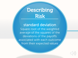
Risk is not only about the average outcome but also about how much outcomes can vary. The standard deviation is a common measure of risk, capturing the extent to which actual outcomes deviate from the expected value.

• Deviation: The difference between an actual payoff and the expected value.

• Variance: The probability-weighted average of the squared deviations from the expected value.

• Standard Deviation: The square root of the variance, providing a measure of risk in the same units as the payoffs.

Formula for Variance ($\sigma^2$):

$\sigma^2 = \sum_{i=1}^{n} P_i (V_i - EV)^2$

Formula for Standard Deviation ($\sigma$):

$\sigma = \sqrt{\sum_{i=1}^{n} P_i (V_i - EV)^2}$

Example: Comparing Job Incomes

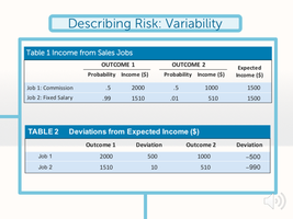
Suppose you are choosing between two part-time jobs with the same expected income but different risk profiles. Job 1 is commission-based, while Job 2 offers a fixed salary. The variability of outcomes is higher for the commission job, as shown by a higher standard deviation.

Job	Outcome 1 Probability/Income	Outcome 2 Probability/Income	Expected Income ($)
Job 1: Commission	0.5 / 2000	0.5 / 1000	1500
Job 2: Fixed Salary	0.99 / 1510	0.01 / 510	1500

Job	Outcome 1 Deviation	Outcome 2 Deviation
Job 1	500	-500
Job 2	10	-990

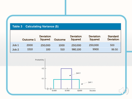
Calculating variance and standard deviation for each job helps quantify the riskiness of each income stream.

Job	Outcome 1 Deviation Squared	Outcome 2 Deviation Squared	Standard Deviation
Job 1	250,000	250,000	500
Job 2	100	980,100	99.50

Examples of Uncertainty

Concert Promoter Example

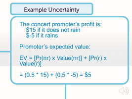
Consider a concert promoter whose profits depend on the weather. If it does not rain, the profit is $15; if it rains, the profit is -$5. Each outcome has a probability of 0.5. The expected value is calculated as follows:

$EV = (0.5 \times 15) + (0.5 \times (-5)) = 5$

Value of Perfect Information

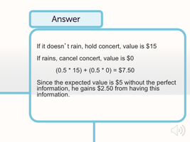
If the promoter could obtain perfect information about the weather, they could avoid losses by only holding the concert if it does not rain. In this case, the expected value increases:

• If it does not rain, hold concert: value = $15

• If it rains, cancel concert: value = $0

$EV = (0.5 \times 15) + (0.5 \times 0) = 7.50$

The value of perfect information is the difference: $7.50 - $5.00 = $2.50.

Preferences Toward Risk

Attitudes Toward Risk

Individuals differ in their willingness to bear risk. Economists classify risk preferences into three categories:

• Risk Averse: Prefers a certain income to a risky income with the same expected value; unwilling to make a fair bet.

• Risk Neutral: Indifferent between a certain income and a risky income with the same expected value; willing to make a fair bet.

• Risk Loving (Risk Preferring): Prefers a risky income to a certain income with the same expected value; seeks out fair bets.

Risk Aversion and Utility

Most people are risk averse. Their utility function is concave with respect to wealth, meaning that each additional dollar increases utility by a smaller amount. A risk-averse individual will choose a less risky option if both choices have the same expected value, and will only choose a riskier option if its expected value is sufficiently higher.

• Concave Utility Function: Utility rises with wealth but at a diminishing rate.

• Expected Utility: The probability-weighted average of the utility of each possible outcome.

Example: If Irma has $40, her utility is 120. She can buy a vase worth $10 (prob. 0.5) or $70 (prob. 0.5). The expected value is $40, but the expected utility is less than the utility of $40, illustrating risk aversion.

$EU = 0.5 \times U(10) + 0.5 \times U(70) = 105$

Since 120 > 105, Irma prefers the certain $40 to the risky alternative.

Summary Table: Risk Attitudes

Type	Preference	Utility Function Shape
Risk Averse	Prefers certainty	Concave
Risk Neutral	Indifferent	Linear
Risk Loving	Prefers risk	Convex

Additional info:

Behavioral economics, which is mentioned as a topic in the lecture, studies how psychological factors and cognitive biases affect economic decision-making under uncertainty. This field extends traditional models by considering that individuals may not always act rationally when facing risk.