9.8: The Unit Circle and the Functions of Trigonometry – Harmonic and Damped Oscillatory Motion

9.8 Harmonic Motion and Trigonometric Functions

Introduction to Simple Harmonic Motion

Simple harmonic motion describes periodic oscillations, such as those seen in springs, pendulums, and waves. This type of motion is fundamental in physics and engineering, and its mathematical model is closely tied to trigonometric functions.

• Simple Harmonic Motion (SHM): The repetitive movement back and forth through an equilibrium position, described by sine or cosine functions.

• Applications: Sound waves, electric currents, and electromagnetic waves all exhibit harmonic motion.

Geometric Representation of Harmonic Motion

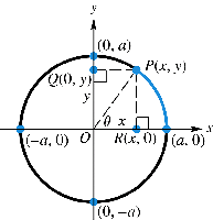
Harmonic motion can be visualized using the unit circle. As a point moves around the circle at a constant angular speed, its projections onto the axes oscillate sinusoidally.

• Unit Circle Model: Let point P(x, y) move counterclockwise around a circle of radius a at a constant angular speed \omega.

• The coordinates of P at time t are:

$x = a \cos(\omega t)$ $y = a \sin(\omega t)$

• As P moves, the projections Q(0, y) and R(x, 0) oscillate between their maximum and minimum values, modeling SHM.

Key Properties of Simple Harmonic Motion

Several important quantities describe the characteristics of harmonic motion:

• Amplitude (|a|): The maximum displacement from equilibrium.

• Period (T): The time for one complete oscillation.

• Frequency (f): The number of cycles per unit time, given by $f = \frac{1}{T}$.

Mathematical Model of Simple Harmonic Motion

The position of an object in SHM at time t can be modeled by:

$s(t) = a \cos(\omega t)$ $s(t) = a \sin(\omega t)$

• Where a is the amplitude, \omega is the angular frequency (\omega > 0), period $T = \frac{2\pi}{\omega}$, and frequency $f = \frac{\omega}{2\pi}$.

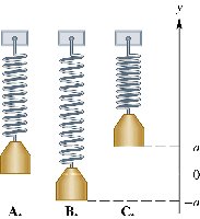
Modeling the Motion of a Spring

Example: Spring-Mass System

Suppose an object is attached to a spring, pulled down 5 units from equilibrium, and released. The period of oscillation is 4 seconds.

• Initial Condition: At t = 0, the displacement is -5 (below equilibrium), so $s(0) = -5$.

• We use the cosine model: $s(t) = a \cos(\omega t)$ with $a = -5$.

• Period $T = 4$, so $\omega = \frac{2\pi}{T} = \frac{2\pi}{4} = \frac{\pi}{2}$.

• Equation: $s(t) = -5 \cos\left(\frac{\pi}{2} t\right)$

• Position at t = 1.5 s:

$s(1.5) = -5 \cos\left(\frac{\pi}{2} \times 1.5\right) = -5 \cos\left(\frac{3\pi}{4}\right) \approx 3.54$

• The object is above the equilibrium position at this time.

• Frequency: $f = \frac{1}{T} = \frac{1}{4}$ oscillations per second.

Analyzing Harmonic Motion

General Analysis

Given a model $s(t) = a \cos(\omega t)$ or $s(t) = a \sin(\omega t)$, we can determine:

• Amplitude: $|a|$ (maximum displacement)

• Period: $T = \frac{2\pi}{\omega}$

• Frequency: $f = \frac{\omega}{2\pi}$

For example, if $s(t) = 8 \cos(\omega t)$, the amplitude is 8 feet, and the period and frequency are found as above.

Damped Oscillatory Motion

Introduction to Damping

In real systems, friction or resistance causes the amplitude of oscillations to decrease over time. This is called damped oscillatory motion. The motion eventually ceases as energy is lost to the environment.

• Damped Model: $y = e^{-x} \sin x$ or $y = e^{-x} \cos x$

• The exponential factor $e^{-x}$ causes the amplitude to decrease as x increases.

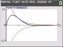
Graphical Analysis of Damped Motion

Consider the function $y = e^{-x} \cos(2\pi x)$. The graph is bounded above and below by the envelopes $y = e^{-x}$ and $y = -e^{-x}$.

• The oscillatory part $\cos(2\pi x)$ causes the function to cross the x-axis periodically.

• The exponential envelope shrinks the amplitude over time.

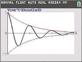
Envelope and Intersection Analysis

• Envelope: The graph of $y = e^{-x} \cos(2\pi x)$ is always between $y = e^{-x}$ and $y = -e^{-x}$.

• Touch Points: The graph touches the upper envelope when $\cos(2\pi x) = 1$, i.e., at $x = 0, 1, 2, 3, \ldots$

• X-axis Intersections: The graph crosses the x-axis when $\cos(2\pi x) = 0$, i.e., at $x = 0.25, 0.75, 1.25, \ldots$

Additional info: Damped oscillatory motion is important in engineering (e.g., shock absorbers, electrical circuits) and physics, where energy dissipation is present.