Graphing Polynomial Functions and Building Cubic Models

Polynomial and Rational Functions

Graphing Polynomial Functions

Polynomial functions are algebraic expressions involving powers of x with real coefficients. Understanding their graphs is essential for analyzing their behavior and solving real-world problems.

• End Behavior: The end behavior of a polynomial function describes how the function behaves as x approaches positive or negative infinity. It is determined by the leading term (the term with the highest degree).

• Intercepts: The y-intercept is found by evaluating the function at x = 0. The x-intercepts (or zeros) are found by solving f(x) = 0.

• Multiplicity of Zeros: The multiplicity of a zero affects whether the graph crosses or merely touches the x-axis at that point. If the zero has an odd multiplicity, the graph crosses the axis; if even, it touches and turns around.

• Turning Points: A polynomial of degree n can have at most n - 1 turning points (local maxima or minima).

• Graph Construction: Use all the above information, plus additional points if needed, to sketch the graph accurately.

Example: Consider the function $f(x) = (x + 1)^3(x - 3)$. Its end behavior resembles $y = x^4$, it crosses the x-axis at $x = -1$ and $x = 3$, and the y-intercept is at $x = 0$.

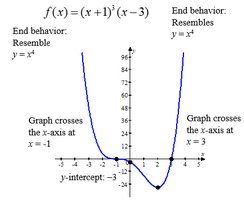
Steps for Graphing a Polynomial Function

1. Determine the end behavior of the graph of the function.

2. Find the x- and y-intercepts of the graph of the function.

3. Determine the zeros of the function and their multiplicity. Use this information to determine whether the graph crosses or touches the x-axis at each x-intercept.

4. Determine the maximum number of turning points on the graph of the function.

5. Use the information in Steps 1 through 4 to draw a complete graph of the function. To help establish the y-axis scale, find additional points on the graph on each side of any x-intercept.

Graphing Polynomial Functions Using a Graphing Utility

Graphing utilities (such as graphing calculators) are powerful tools for analyzing polynomial functions, especially those of higher degree or with complicated coefficients.

• Graphing: Enter the polynomial into the utility to view its graph.

• Finding Intercepts: Use the utility's 'Zero' or 'Root' feature to approximate x-intercepts, and evaluate at x = 0 for the y-intercept.

• Tables: Generate tables of values to examine the function's behavior near intercepts and turning points.

• Turning Points: Use 'Maximum' and 'Minimum' features to locate local extrema.

• Domain and Range: The domain of a polynomial function is all real numbers. The range can be estimated from the graph.

• Intervals of Increase/Decrease: Determine where the function is increasing or decreasing by analyzing the graph.

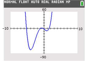
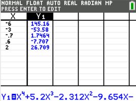
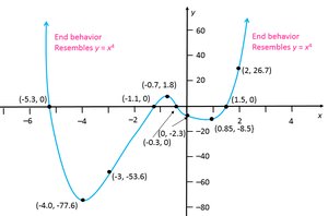
Summary: Steps for Using a Graphing Utility

1. Determine the end behavior of the graph of the function.

2. Graph the function using a graphing utility.

3. Use a graphing utility to approximate the x- and y-intercepts of the graph.

4. Use a graphing utility to create a Table to find points on the graph around each x-intercept.

5. Approximate the turning points of the graph.

6. Use the information in Steps 1 through 5 to draw a complete graph of the function by hand.

7. Find the domain and the range of the function.

8. Use the graph to determine where the function is increasing and where it is decreasing.

Building Cubic Models from Data

Polynomial models, especially cubic functions, are useful for fitting data that exhibit non-linear trends. A cubic model has the form $y = ax^3 + bx^2 + cx + d$.

• Scatter Diagram: Plot the data points to visually assess the relationship between variables.

• Cubic Regression: Use a graphing utility to perform cubic regression and find the best-fit cubic function for the data.

• Model Interpretation: The resulting cubic function can be used to make predictions and analyze trends.

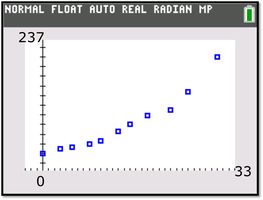
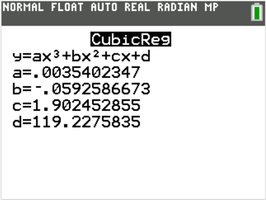
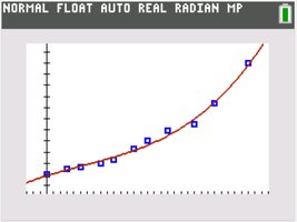
Example: Predicting Costs with a Cubic Model

Suppose the weekly cost C (in thousands of dollars) of printing x thousand books is modeled by a cubic function found via regression. To predict the cost for a specific value of x, substitute into the model and compute the result.

• Given: $C(x) = 0.00354x^3 - 0.05926x^2 + 1.90245x + 119.2276$

• To predict the cost for 20 thousand books:

$C(20) = 0.00354 \times 20^3 - 0.05926 \times 20^2 + 1.90245 \times 20 + 119.2276 \approx 161.9$

The model predicts a cost of $161,900 for printing 20,000 books in a week.