Parametric and Implicit Functions in Precalculus: Concepts, Applications, and Examples

Section 6.2: Parametric and Implicit Functions Revisited

Introduction to Parametric Curves

Parametric equations provide a way to represent curves by expressing both x and y as functions of a third variable, called the parameter (usually t). This approach is especially useful for describing the motion of objects and curves that cannot be represented as functions in the form y = f(x).

• Parametric Curve: The set of ordered pairs (x, y) where $x = f(t)$ and $y = g(t)$ for $t$ in an interval $I$.

• Parameter Interval: The set of values for $t$ over which the functions are defined.

• Applications: Modeling the path of objects (e.g., baseballs, golf balls), describing motion, and representing curves not easily written as explicit functions.

Graphing Parametric Functions

Example: Graphing a Parametric Function

To graph a parametric function, plot the points $(x(t), y(t))$ for values of $t$ in the parameter interval. Adjust the viewing window on a graphing calculator to ensure the curve is fully visible.

• Calculator Settings: Set $T_{min}$, $T_{max}$, and $T_{step}$ to control the parameter range and step size. Adjust $X_{min}$, $X_{max}$, $Y_{min}$, and $Y_{max}$ for the viewing window.

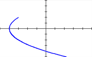
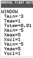
Do Textbook problems page 488 #17-20.

Eliminating the Parameter

Converting Parametric Equations to Cartesian Form

To analyze or graph a parametric curve using standard methods, it is often useful to eliminate the parameter and obtain a single equation relating $x$ and $y$.

• Step 1: Solve one of the parametric equations for $t$.

• Step 2: Substitute this expression for $t$ into the other equation to obtain a relationship between $x$ and $y$.

• Result: The resulting equation describes the same curve in the $xy$-plane.

• Example: If $x = 5 - t^2$ and $y = 2t$, solve for $t$ in terms of $y$ ($t = y/2$), substitute into $x$, and obtain $x = 5 - (y/2)^2$.

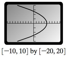
Additional info: The resulting equation $x = 5 - (y/2)^2$ is a parabola opening to the left with vertex at (5, 0).

Do Textbook problems page 488 #21-30 (multiples of 3) and #33-36.

Parametric Equations for Line Segments

Finding a Parametric Representation

A line segment between two points $A(x_1, y_1)$ and $B(x_2, y_2)$ can be represented parametrically by expressing the coordinates as linear functions of $t$, where $t$ varies from 0 to 1.

• Formulas: $x = x_1 + (x_2 - x_1)t$ $y = y_1 + (y_2 - y_1)t$ for $0 \leq t \leq 1$

• Example: For $A(2, 3)$ and $B(-3, 6)$: $x = 2 - 5t$ $y = 3 + 3t$ for $0 \leq t \leq 1$

When $t = 0$, the point is at $A$; when $t = 1$, the point is at $B$.

Do textbook problems page 488 #37-40.

Applications: Projectile Motion

Modeling the Path of a Baseball

Parametric equations are used to model the motion of projectiles, such as a baseball hit at an angle. The horizontal and vertical positions are given by:

• $x(t) = v_0 \cos(\theta) t$

• $y(t) = y_0 + v_0 \sin(\theta) t - \frac{1}{2}gt^2$

• where $v_0$ is the initial velocity, $\theta$ is the launch angle, $y_0$ is the initial height, and $g$ is the acceleration due to gravity (typically 32$ft/s$^2).

Example: A baseball is hit 4 ft above the ground with an initial velocity of 120 ft/sec at a 30° angle. The equations become:

• $x(t) = 120 \cos(30^\circ) t$

• $y(t) = 4 + 120 \sin(30^\circ) t - 16 t^2$

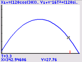
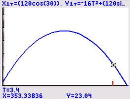
At $t = 3.3$ sec, $x \approx 343$ ft, $y \approx 27.76$ ft; at $t = 3.4$ sec, $x \approx 353$ ft, $y \approx 23.04$ ft. The ball does not clear a 30-ft fence 350 ft away; it hits the wall between these times.

Do textbook problems page 489 #68 and 70-72.

Implicitly and Explicitly Defined Functions

Understanding Implicit and Explicit Forms

Some equations define functions implicitly, such as $Ax + By = C$, which is not solved for $y$. Explicit forms, such as $y = mx + b$, directly express the dependent variable in terms of the independent variable.

• Implicit Form: $Ax + By = C$

• Explicit Form: $y = mx + b$ or $y = m(x - h) + k$

• Advantage: Explicit forms are easier to graph and analyze, and can be entered directly into calculators.

Do textbook problems page 487 #3-4; and page 488 #47-54.

Rates of Change for Parametric Curves

Average Rate of Change

For a curve defined parametrically by $x = f(t)$ and $y = g(t)$, the average rate of change of $y$ with respect to $x$ over $t_1 \leq t \leq t_2$ is:

• $\text{Average rate of change} = \frac{\Delta y}{\Delta x} = \frac{y(t_2) - y(t_1)}{x(t_2) - x(t_1)}$

• This gives the slope of the secant line between the points corresponding to $t_1$ and $t_2$.

Example: If $y$ decreases by 1 unit as x increases by 2 units, the average rate of change is $-\frac{1}{2}$.

Do textbook problems page 488 #57-58.