Study Notes: Linear Functions and Linear Models (Precalculus Chapter 3.1)

Linear Functions and Linear Models

Definition and Properties of Linear Functions

A linear function is a function of the form $f(x) = mx + b$, where m is the slope and b is the y-intercept. The graph of a linear function is a straight line. The domain of a linear function is typically all real numbers, unless otherwise restricted by context.

• Slope (m): Measures the steepness of the line; calculated as the change in y divided by the change in x.

• Y-intercept (b): The value of the function when $x = 0$.

• Domain: Usually $(-\infty, \infty)$ unless context restricts it.

• Nonlinear functions: Functions whose graphs are not straight lines.

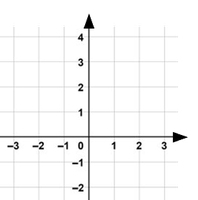
Example: Graphing a linear function on a coordinate plane.

Average Rate of Change and Identification of Linear Functions

The average rate of change of a function between two points $(x_1, y_1)$ and $(x_2, y_2)$ is given by:

$\frac{\Delta y}{\Delta x} = \frac{y_2 - y_1}{x_2 - x_1}$

• For linear functions, the average rate of change is constant for any interval.

• This property can be used to identify whether a function is linear.

Theorem: The average rate of change of a linear function is always equal to its slope, m.

Example: Using a table to compute the average rate of change for $y = f(x) = -3x + 7$.

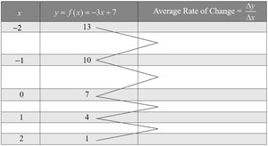
In the table, the average rate of change between any two consecutive x-values is always -3, confirming the function is linear.

Increasing, Decreasing, and Constant Linear Functions

A linear function $f(x) = mx + b$ can be classified based on its slope:

• Increasing: If $m > 0$, the function increases over its domain.

• Decreasing: If $m < 0$, the function decreases over its domain.

• Constant: If $m = 0$, the function is constant (horizontal line).

Example: Determining whether a linear function is increasing, decreasing, or constant by examining its slope.

Building Linear Models from Verbal Descriptions

When the average rate of change between two variables is constant, a linear function can model their relationship. The general form is $f(x) = mx + b$, where m is the rate of change and b is the initial value (value when $x = 0$).

• Modeling: Translate real-world situations into linear equations by identifying the rate of change and initial value.

Example: Straight-line Depreciation

• A company purchases a computer for $3000 and depreciates it over 3 years using the straight-line method.

• The depreciation per year is constant.

• The linear model for book value $V$ as a function of age $x$ is $V(x) = 3000 - mx$, where $m$ is the annual depreciation.

• Domain: $0 \leq x \leq 3$ (since the computer is depreciated over 3 years).

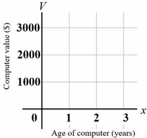
Applications: Find the value after 2 years, or when the value reaches $2000$by solving$V(x) = 2000$.

Supply and Demand: Linear Models in Economics

Linear functions are used to model supply and demand relationships in economics. The equilibrium price is found where the supply and demand functions intersect.

• Supply function: $S(p)$, where $p$ is price.

• Demand function: $D(p)$, where $p$ is price.

• Equilibrium: Occurs when $S(p) = D(p)$.

• Equilibrium quantity: The value of $S(p)$ or $D(p)$ at equilibrium price.

• If quantity demanded is greater than quantity supplied, price tends to rise until equilibrium is reached.

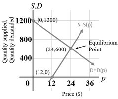
Example: Find equilibrium price and quantity, and analyze what happens when demand exceeds supply.

Additional info: These notes expand on brief points from the original materials, providing definitions, formulas, and context for precalculus students studying linear functions and their applications.