Population Ecology: Principles, Models, and Applications

Population Ecology

Introduction to Population Ecology

Population ecology is the study of populations of organisms, especially their size, structure, distribution, and dynamics over time. It is distinct from community ecology (which examines interactions among species) and ecosystem ecology (which focuses on energy and nutrient flows).

• Population: A group of individuals of the same species living in a defined area.

• Population ecology: Focuses on factors affecting population size and growth.

• Levels of ecological study: Organism, population, community, ecosystem, biosphere.

Population Distributions

Populations can be distributed in space in several characteristic patterns, each reflecting underlying ecological processes.

• Clumped: Individuals aggregate in patches, often due to resource availability or social behavior.

• Uniform: Individuals are evenly spaced, often due to territoriality or competition.

• Random: Individuals are distributed unpredictably, usually when environmental conditions are uniform.

Population Growth Variables and Models

Population growth is described using mathematical models and key variables.

• N: Population size (number of individuals).

• t: Time interval.

• r: Intrinsic rate of increase (per capita growth rate).

• R0: Net reproductive rate (average number of offspring per individual).

Exponential Growth

Exponential growth occurs when resources are unlimited, and the population increases at a constant rate.

• Formula: $\Delta N/\Delta t = rN$

• Characteristics: J-shaped curve; rapid increase.

• Example: If a deer population starts at 500 and r = 0.06, after 1 year: $\Delta N = rN = 0.06 \times 500 = 30$; new population = 530.

Logistic Growth and Carrying Capacity (K)

Logistic growth incorporates environmental limits, resulting in an S-shaped curve as the population approaches carrying capacity (K).

• Formula: $\Delta N/\Delta t = rN \left(1 - \frac{N}{K}\right)$

• Carrying capacity (K): Maximum population size the environment can sustain.

• Example: If K = 600, growth slows as N approaches 600.

Survivorship Curves and Life History Strategies

Survivorship curves graphically represent the proportion of individuals surviving at each age.

• Type I: High survival early, steep decline at old age (e.g., humans).

• Type II: Constant mortality rate across ages (e.g., birds).

• Type III: High mortality early, survivors live long (e.g., many fish).

Life History Strategies

• r-selected species: Rapid reproduction, high fecundity, short lifespan, unstable environments.

• K-selected species: Slow reproduction, low fecundity, long lifespan, stable environments.

Human Population Trends and Age Pyramids

Age pyramids illustrate the age structure of populations and can predict growth trends.

• Wide base: Rapid growth.

• Even shape: Stable population.

• Narrow base: Declining population.

Mark-Recapture Methods

Mark-recapture is a technique for estimating population size by capturing, marking, and recapturing individuals.

• Formula: $N = \frac{n_1 \times n_2}{m_2}$, where n1 = marked initially, n2 = captured later, m2 = marked recaptures.

Key Vocabulary

• Fecundity: Number of offspring produced per individual.

• Natality: Birth rate.

• Recruitment: Addition of new individuals to the population.

• Metapopulation: Group of populations separated by space but connected by dispersal.

• Density-dependent factor: Effects increase with population density (e.g., competition, disease).

Life Table Analysis: White-Tailed Deer (Odocoileus virginianus)

Life Table Interpretation

Life tables summarize survival and reproductive rates by age class, providing insight into population dynamics.

• Fecundity peak: Highest mx value (age 4: mx = 1.4).

• Greatest contribution to growth: Highest lx·mx value (age 4: lx·mx = 0.429).

• Reproduction begins: Age 2 (mx = 0.1).

• Survivorship change: lx drops from 1.0 (birth) to 0.324 (age 2).

• Mortality rate: qx at age 1 = 0.1; age 5 = 0.1.

Quantitative Analysis

• Net Reproductive Rate (R0): $R_0 = \sum (lx \cdot mx) = 2.627$

• Generation Time (T): $T = \frac{\sum (x \cdot lx \cdot mx)}{\sum (lx \cdot mx)}$

• Harvest strategy: Target age class with highest lx·mx (age 4) to reduce growth.

Conceptual Thinking

• Survivorship curve: Data suggests Type I/II (moderate juvenile survival, gradual decline).

• K-selected vs r-selected: Deer are more K-selected (long lifespan, parental care, moderate fecundity).

• Predation on fawns: Increased mortality at age 0–1 lowers R0, reducing population stability.

• Parental care: Increases survivorship, shapes fecundity patterns.

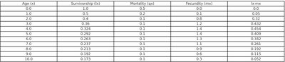
Life Table for Female White-Tailed Deer

Age (x)	Survivorship (lx)	Mortality (qx)	Fecundity (mx)	lx·mx
0.0	1.0	0.5	0.0	0.0
1.0	0.5	0.1	0.2	0.1
2.0	0.324	0.1	0.1	0.032
3.0	0.294	0.1	1.1	0.324
4.0	0.294	0.1	1.4	0.429
5.0	0.263	0.1	1.3	0.342
6.0	0.217	0.1	1.1	0.239
7.0	0.174	0.1	0.8	0.139
8.0	0.139	0.1	0.7	0.097
9.0	0.111	0.1	0.7	0.078
10.0	0.078	0.1	0.7	0.055

Data Extensions

• Survivorship curve: Plot lx values; curve shows gradual decline, typical of Type I/II.

• Fecundity curve: Plot mx values; fecundity peaks at age 4, declines after age 7.

• R0 < 1: Implies population decline; table could be adjusted by lowering mx or increasing qx.

Regulation of Populations: Top-Down vs Bottom-Up

Definitions

• Top-down regulation: Population controlled by predators, parasites, or disease.

• Bottom-up regulation: Population controlled by resource availability (food, water, shelter).

Concept Questions

• If deer increase despite predators, top-down regulation is ineffective.

• Drop in birth rates after harsh winter is bottom-up regulation.

• Stable deer numbers despite fewer predators may be due to resource limitation or other density-dependent factors.

• Density-dependent top-down: predation by wolves; bottom-up: food scarcity in winter.

Population Cycles in Deer and Predators

Predator-Prey Dynamics

Population cycles often occur between prey and predator species, with predator numbers lagging behind prey.

• Trend: Deer population rises, then falls as wolf population increases; wolf numbers lag behind deer.

• Predator-prey cycles: Evidence of cycling similar to hare–lynx model.

• Time lag: Wolf population increases after deer population peaks.

• Bottom-up pressure: Food shortage in 2017 could explain deer decline.

Graphing Population Cycles

• Graph deer and wolf populations over time; predator numbers follow prey dynamics.

Additional info: Academic context was added to clarify formulas, definitions, and ecological principles for completeness.