lec 24

Population Genetic Structure and Inbreeding

Hardy-Weinberg Equilibrium (HWE) and Its Assumptions

The Hardy-Weinberg Equilibrium (HWE) provides a foundational model for understanding allele and genotype frequencies in populations. It assumes that allele frequencies remain constant from generation to generation in the absence of evolutionary influences.

• No selection: Alleles are not adaptive; all genotypes have equal fitness.

• No mutation: No new alleles are introduced via mutation.

• No genetic drift: Population size is large enough to prevent random changes in allele frequencies.

• No non-random mating: Mating is completely random; every individual has an equal chance to mate with any other of the opposite sex.

• No migration: No new alleles are introduced by movement of individuals between populations.

Non-Random Mating and Inbreeding

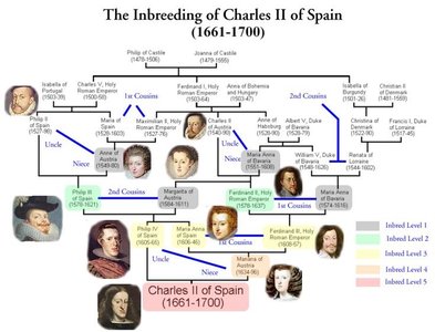
Non-random mating occurs when individuals do not mate at random, often due to physical, social, or environmental factors. Inbreeding is a specific form of non-random mating where closely related individuals mate, increasing the probability that offspring inherit identical alleles by descent.

• Inbreeding: Mating between relatives (siblings, cousins, etc.), leading to increased homozygosity and decreased heterozygosity.

• Hermaphroditic reproduction: Organisms capable of self-fertilization (selfing) rapidly reduce heterozygosity in a population.

Effects of Selfing on Heterozygosity

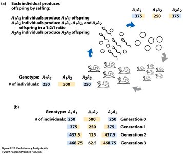
Self-fertilization (selfing) is an extreme form of inbreeding. It causes a rapid decline in heterozygosity, while allele frequencies remain unchanged.

• Each generation of selfing halves the proportion of heterozygotes.

• Homozygosity increases correspondingly.

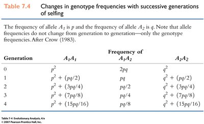
Generation	Frequency of A1A1	Frequency of A1A2	Frequency of A2A2
0	p2	2pq	q2
1	p2 + (pq/2)	pq	q2 + (pq/2)
2	p2 + (3pq/4)	pq/2	q2 + (3pq/4)
3	p2 + (7pq/8)	pq/4	q2 + (7pq/8)
4	p2 + (15pq/16)	pq/8	q2 + (15pq/16)

Additional info: Table shows how genotype frequencies change with each generation of selfing, but allele frequencies (p and q) remain constant.

Coefficient of Inbreeding (F)

The coefficient of inbreeding (F) quantifies the probability that two alleles in an individual are identical by descent. It is incorporated into Hardy-Weinberg models to predict genotype frequencies in inbred populations.

• Homozygote frequency: $p^2(1-F) + pF$ for A1A1, $q^2(1-F) + qF$ for A2A2

• Heterozygote frequency: $2pq(1-F)$ for A1A2

• Heterozygosity in inbred population: $H_F = H_O (1-F)$

Additional info: F ranges from 0 (no inbreeding) to 1 (complete inbreeding, as in selfing).

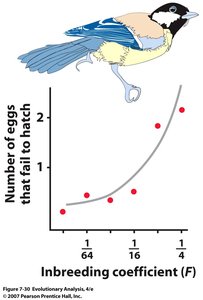
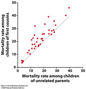
Inbreeding Depression

Inbreeding depression is the reduction in fitness due to increased homozygosity, which exposes deleterious recessive alleles to selection. It is measured as:

• $d = 1 - \frac{w_S}{w_O}$, where $w_S$ is the fitness of inbred individuals and $w_O$ is the fitness of outbred individuals.

• Common in plants due to frequent selfing and proximity of relatives.

Population Genetics and Conservation

Wright’s F-Statistics

Wright’s F-statistics are used to quantify population genetic structure and the effects of non-random mating. The most commonly used statistic is $F_{ST}$, which measures genetic differentiation among subpopulations.

• F: General inbreeding coefficient.

• FST: Proportion of genetic variance among subpopulations relative to the total genetic variance.

• Calculation: $2pq(1-F) = \text{observed heterozygote frequency}$

Example Calculation:

• Given $p = 0.6$, $q = 0.4$, observed heterozygote frequency = 0.375

• $2(0.6)(0.4)(1-F) = 0.375$

• $0.48(1-F) = 0.375$

• $1-F = 0.375/0.48 = 0.78$

• $F = 1 - 0.78 = 0.22$

Additional info: Higher FST values indicate greater genetic differentiation among populations.

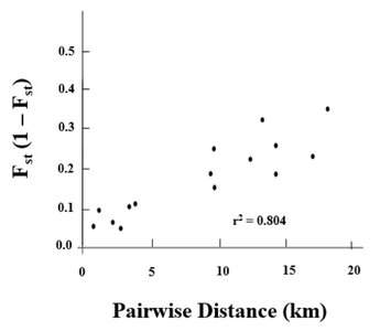
Isolation by Distance (IBD) and Isolation by Environment (IBE)

Population genetic structure can be influenced by spatial and environmental factors:

• Isolation by Distance (IBD): Genetic differentiation increases with geographic distance due to limited gene flow and genetic drift.

• Isolation by Environment (IBE): Genetic differentiation correlates with environmental differences, often due to natural selection acting on populations in different habitats.

Species Distribution Modeling (SDM)

Species distribution models use environmental data (climate layers) to predict where suitable habitat for a species is likely to occur. These models are important for understanding how genetic structure may be shaped by both geography and environment.

• Environmental variables: Temperature, precipitation, seasonality, etc.

• Applications: Predicting species ranges, identifying conservation priorities, and understanding the effects of climate change on genetic diversity.

Summary Table: Key Equations and Concepts

Concept	Equation	Description
Heterozygosity under inbreeding	$H_F = H_O (1-F)$	Heterozygosity decreases with inbreeding coefficient F
Inbreeding depression	$d = 1 - \frac{w_S}{w_O}$	Reduction in fitness due to inbreeding
Genotype frequencies with inbreeding	$A_{11}: p^2(1-F) + pF$ $A_{12}: 2pq(1-F)$ $A_{22}: q^2(1-F) + qF$	Genotype frequencies in an inbred population
Wright's FST	$F_{ST} = 1 - \frac{H_S}{H_T}$	Genetic differentiation among subpopulations

Applications in Conservation Biology

Understanding population genetic structure and the effects of inbreeding is critical for conservation biology. Loss of genetic diversity can increase extinction risk, reduce adaptability, and cause inbreeding depression in small or fragmented populations.

• Genetic monitoring can inform management strategies to maintain or restore genetic diversity.

• Species distribution models help identify suitable habitats and prioritize areas for conservation.