Speciation, Hardy–Weinberg Principle, and Phylogenetic Trees: Study Notes

Speciation and Evolutionary Processes

Hardy–Weinberg Principle: Mathematical Null Hypothesis for Evolution

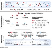
The Hardy–Weinberg principle provides a mathematical framework to study evolutionary processes by predicting allele and genotype frequencies in a population under specific conditions. It serves as a null hypothesis, allowing biologists to detect deviations caused by evolutionary forces.

• Allele Frequencies: For a gene with two alleles (A1 and A2), their frequencies are denoted as p and q, respectively. The sum of allele frequencies is $p + q = 1$.

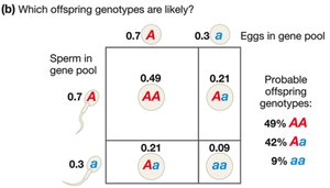
• Genotype Frequencies: Three genotypes are possible: A1A1, A1A2, and A2A2. Their frequencies are predicted by the equation $p^2 + 2pq + q^2 = 1$.

• Hardy–Weinberg Equation: $p^2$ = frequency of A1A1 genotype $2pq$ = frequency of A1A2 genotype $q^2$ = frequency of A2A2 genotype

• Assumptions: The model assumes random mating, no natural selection, no genetic drift, no gene flow, and no mutation.

Testing Hardy–Weinberg Equilibrium

To determine if a population is in Hardy–Weinberg equilibrium, biologists follow four steps:

1. Estimate genotype frequencies from sample data.

2. Calculate observed allele frequencies from genotype frequencies.

3. Use observed allele frequencies to calculate expected genotype frequencies using Hardy–Weinberg equations.

4. Statistically compare observed and expected values to assess equilibrium.

Example Calculations

Consider a population of lizards with three genotypes: GG, Gg, and gg. To calculate allele frequencies:

• Frequency of G = frequency of GG + ½ frequency of Gg

• Frequency of g = frequency of gg + ½ frequency of Gg

Expected genotype frequencies under Hardy–Weinberg equilibrium are calculated using the observed allele frequencies.

Speciation: Formation of New Species

Overview of Speciation

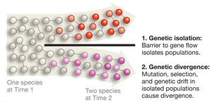
Speciation is the evolutionary process by which new biological species arise. It involves two main steps:

• Genetic Isolation: A barrier to gene flow isolates populations within a species.

• Genetic Divergence: Mutation, natural selection, and genetic drift cause populations to diverge genetically.

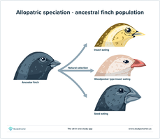
Allopatric Speciation

Allopatric speciation occurs when populations become geographically separated, leading to genetic isolation and divergence.

• Dispersal: Movement of individuals to a new location.

• Vicariance: Physical splitting of a habitat by a barrier.

Sympatric Speciation

Sympatric speciation occurs within populations living in the same geographic area. It can be initiated by:

• External (extrinsic) events: Disruptive selection based on ecological niches or mate preferences.

• Internal (intrinsic) events: Chromosomal mutations, such as polyploidy.

Example: Killer whales form distinct ecotypes within the same ocean, separated by feeding culture (extrinsic event).

Example: Bread wheat evolved through hybridization and chromosomal doubling (intrinsic event).

Species Concepts: Defining and Identifying Species

The Biological Species Concept

Species are defined by reproductive isolation, which prevents gene flow between populations.

• Prezygotic isolation: Prevents mating or fertilization.

• Postzygotic isolation: Hybrid offspring are inviable or sterile.

The Morphological Species Concept

Species are distinguished by differences in morphological features. Useful for sexual, asexual, and fossil species, but may misclassify polymorphic or cryptic species.

The Phylogenetic Species Concept

Species are identified based on evolutionary history and common ancestry. Monophyletic groups (clades) include an ancestor and all its descendants.

Phylogenetic Trees: Evolutionary Relationships

Structure and Interpretation of Phylogenetic Trees

Phylogenetic trees depict the evolutionary history of organisms. Key features include:

• Taxa: Groups of organisms at branch tips.

• Nodes: Branching points representing common ancestors.

• Sister taxa: Groups sharing a most recent common ancestor.

Estimating Phylogenies

Biologists use genetic and morphological data to estimate phylogenies. Sequence comparisons and character matrices help determine relationships.

• Ancestral traits: Traits present in ancestors.

• Derived traits: Modified traits found in descendants.

Monophyletic Groups and Synapomorphies

Monophyletic groups (clades) are identified by shared derived traits (synapomorphies). Other terms include:

• Apomorphy: Derived trait.

• Autapomorphy: Derived in a single lineage.

• Plesiomorphy: Ancestral trait.

Complications in Phylogenetic Inference

Traits may be similar due to homoplasy (independent evolution) rather than homology (common ancestry). Parsimony is used to select the tree with the fewest evolutionary changes.

Summary Table: Species Concepts

Concept	Main Criterion	Advantages	Disadvantages
Biological Species Concept	Reproductive isolation	Directly relates to gene flow	Not applicable to asexual/fossil species
Morphological Species Concept	Distinct morphological features	Widely applicable	Subjective; may misclassify
Phylogenetic Species Concept	Common ancestry; monophyletic groups	Objective; evolutionary history	Requires extensive data

Summary Table: Hardy–Weinberg Calculations

Population	Genotype Frequencies (AA, AC, CC)	Allele Frequencies (A, C)
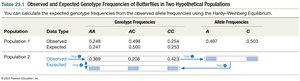
Population 1 (Observed)	0.247, 0.498, 0.254	0.497, 0.503
Population 2 (Observed)	0.369, 0.208, 0.423	0.473, 0.527
Population 2 (Expected)	0.224, 0.499, 0.278	0.473, 0.527

Key Equations

• Allele frequency: $p + q = 1$

• Genotype frequency: $p^2 + 2pq + q^2 = 1$