Ch. 9 - Differential Equations
Briggs - Calculus: Early Transcendentals 3rd Edition
Briggs3rd EditionCalculus: Early TranscendentalsISBN: 9780136847243당신이 사용하는 게 아니라요?교과서 변경
9장, 문제 9.5.1

Explain how the growth rate function determines the solution of a population model.

검증된 단계별 안내
1
Understand that in population models, the growth rate function describes how the population changes over time, often expressed as a function of the current population size, say \(r(P)\), where \(P\) is the population at time \(t\).
Recognize that the population model is typically formulated as a differential equation of the form \(\frac{dP}{dt} = r(P) \cdot P\), where \(\frac{dP}{dt}\) represents the rate of change of the population with respect to time.
Analyze how the form of the growth rate function \(r(P)\) influences the behavior of the solution: for example, if \(r(P)\) is constant and positive, the population grows exponentially; if \(r(P)\) decreases as \(P\) increases, it may model limited resources leading to logistic growth.
Solve the differential equation by separating variables or using an integrating factor, depending on the form of \(r(P)\), to find the explicit solution \(P(t)\) that describes the population at any time \(t\).
Interpret the solution \(P(t)\) in terms of the growth rate function to understand long-term behavior such as equilibrium points, carrying capacity, or unbounded growth, which are all determined by the characteristics of \(r(P)\).

비슷한 문제에 대한 검증된 영상 답변:

이 영상 해법은 위 문제에 도움이 된다고 튜터들이 추천한 것입니다.
영상 길이:
3m
도움이 되었나요?

주요 개념

질문에 올바르게 답하기 위해 반드시 이해해야 하는 핵심 개념들은 다음과 같습니다.

Growth Rate Function

The growth rate function describes how the population changes over time, often expressed as a rate of change dependent on the current population size. It can be constant or vary with population, influencing whether the population grows, declines, or stabilizes.
추천 영상:
04:16
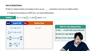
Intro To Related Rates

Differential Equations in Population Models

Population models are typically formulated as differential equations where the growth rate function defines the derivative of the population with respect to time. Solving these equations provides the population size as a function of time, revealing the dynamics of growth.
추천 영상:
07:39
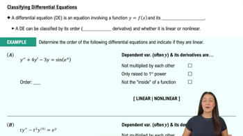
Classifying Differential Equations

Equilibrium Solutions and Stability

Equilibrium solutions occur when the growth rate is zero, indicating a stable or unstable population size. Analyzing these points helps predict long-term behavior of the population, such as whether it will settle at a steady state or experience unbounded growth or decline.
추천 영상:
04:00
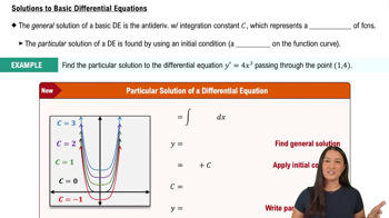
Solutions to Basic Differential Equations
관련 실천
교과서 질문

17–32. Solving initial value problems Determine whether the following equations are separable. If so, solve the initial value problem.

y'(t) = y³sin t, y(0) = 1

59
views

교과서 질문

7–16. Verifying general solutions Verify that the given function is a solution of the differential equation that follows it. Assume C, C1, C2 and C3 are arbitrary constants.

u(t) = C₁eᵗ + C₂teᵗ; u''(t) - 2u'(t) + u(t) = 0

41
views
교과서 질문

The general solution of a first-order linear differential equation is y(t) = Ce⁻¹⁰ᵗ − 13. What solution satisfies the initial condition y(0) = 4?

84
views
교과서 질문

9–14. Growth rate functions Make a sketch of the population function P (as a function of time) that results from the following growth rate functions. Assume the population at time t = 0 begins at some positive value.


22
views
교과서 질문

9–14. Growth rate functions Make a sketch of the population function P (as a function of time) that results from the following growth rate functions. Assume the population at time t = 0 begins at some positive value.


39
views
교과서 질문

45–48. General first-order linear equations Consider the general first-order linear equation y'(t)+a(t)y(t)=f(t). This equation can be solved, in principle, by defining the integrating factor p(t)=exp(∫a(t)dt). Here is how the integrating factor works. Multiply both sides of the equation by p (which is always positive) and show that the left side becomes an exact derivative. Therefore, the equation becomes


p(t)(y′(t) + a(t)y(t)) = d/dt(p(t)y(t)) = p(t)f(t).


Now integrate both sides of the equation with respect to t to obtain the solution. Use this method to solve the following initial value problems. Begin by computing the required integrating factor.


y′(t) + (2t)/(t² + 1)y(t) = 1 + 3t², y(1) = 4

75
views