Aggregate Demand and Aggregate Supply Analysis: Macroeconomics Study Notes

Chapter 13: Aggregate Demand and Aggregate Supply Analysis

Introduction

This chapter explores the aggregate demand and aggregate supply model, a fundamental framework in macroeconomics used to analyze short-run fluctuations in real GDP, employment, and the price level. The chapter covers the determinants and dynamics of aggregate demand and supply, macroeconomic equilibrium, and the main schools of thought in macroeconomic theory.

• AD - AS Framework model, explains short-run fluctuations in real GDP and price level

Aggregate Demand (Real GDP or Total spending on goods/services in an economy)

Determinants of Aggregate Demand

Aggregate demand (AD) represents the total quantity of goods and services demanded across the economy at different price levels. It is composed of four main components:

• Consumption (C): Spending by households on goods and services.

• Investment (I): Spending by firms on capital goods.

• Government Purchases (G): Expenditures by government on goods and services (independent of changes in the price level, causes a shift on the curve)

• Net Exports (NX): Exports minus imports.

• Consumption, investment and net exports are affected by changes in the price level.

• The aggregate demand (AD)curve shows the relationship between the price level and the quantity of real GDP demanded by households, firms, and the government (both inside and outside of the country.)

• Short-run aggregate supply (SRAS) curve shows the relationship in the short run between the price level and the quantity of real GDP supplied by firms

Effects of Price Level Changes

• Wealth Effect: As price levels rise, the real value of household wealth declines, leading to reduced consumption (some is held in nominal assets, fixed terms that does not adjust for inflation like cash)

• Interest-Rate Effect: Higher price levels increase the demand for money, raising interest rates and discouraging investment.

• International-Trade Effect: Higher U.S. price levels make exports more expensive and imports cheaper, reducing net exports.

These effects explain why the aggregate demand curve slopes downward.

Movements vs. Shifts of the Aggregate Demand Curve

• Movement along the AD curve: Caused by changes in the price level, holding other factors constant (C,I, NX)

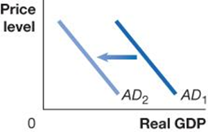
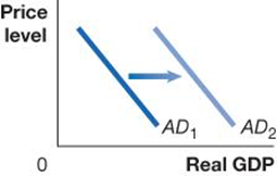
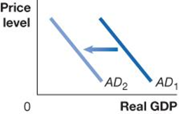
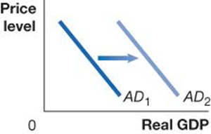
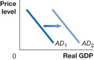
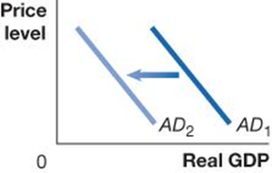
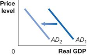
• Shift of the AD curve: Caused by changes in any component of real GDP (C, I, G, NX) due to factors other than the price level.

Variables That Shift the Aggregate Demand Curve

• Monetary Policy: Actions by the Federal Reserve affecting money supply and interest rates. Higher interest rates decrease investment spending, shifting AD left; lower rates increase investment, shifting AD right.

• Fiscal Policy: Changes in taxes and government purchases. Increased government spending or lower taxes shift AD right b/c there's an increase in GDP; decreased spending or higher taxes shift AD left.

• It can also alter business taxes, affecting the level of investment spending

• Expectations: Optimism among households or firms increases consumption and investment, shifting AD right; pessimism shifts AD left.

• Foreign Variables: Changes in foreign income or exchange rates affect net exports. Higher foreign income increases U.S. exports, shifting AD right; a stronger dollar reduces exports, shifting AD left.

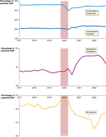
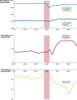
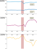
Aggregate Demand During the 2020 Recession

• Consumption: Fell sharply, especially in services.

• Investment: Residential investment increased due to low interest rates and stimulus checks.

• Net Exports: Decreased due to a stronger dollar and lower foreign demand.

Aggregate Supply

Determinants of Aggregate Supply

Aggregate supply (AS) is the total quantity of goods and services firms are willing and able to supply at different price levels. The relationship between price level and real GDP supplied differs in the short run and long run.

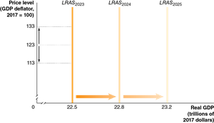
• Long-Run Aggregate Supply (LRAS): Vertical line (|) at potential GDP, determined by labor, capital stock (factories, machinery, etc), and technology. Not affected by price level. LRAS occurs at the level of potential or full-employment GDP, which advances each year.

• Short-Run Aggregate Supply (SRAS): Upward sloping due to sticky wages and prices, slow wage adjustments, and menu costs. /

Why Is the SRAS Curve Upward Sloping?

• Sticky Wages and Prices: Contracts and slow adjustments make wages and prices less responsive to changes in demand.

• Slow Wage Adjustments: Firms review salaries infrequently and avoid wage cuts.

• Menu Costs: Firms incur costs when changing prices, leading to price stickiness.

Movements vs. Shifts of the SRAS Curve

• Movement along SRAS: Caused by changes in the price level, holding other factors constant.

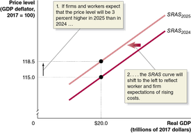
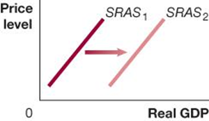
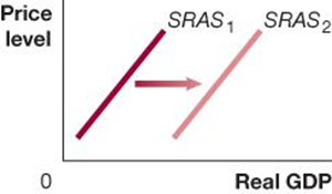
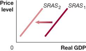
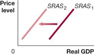
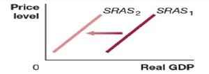
• Shift of SRAS: Caused by changes in factors such as labor, capital, technology, expected future prices, and supply shocks.

Variables That Shift the Short-Run Aggregate Supply Curve

• Labor and Capital: Increased availability shifts SRAS right; decreased availability shifts SRAS left.

• Technology: Improvements shift SRAS right.

• Expected Future Price Level: Higher expected prices shift SRAS left; lower expected prices shift SRAS right.

• Supply Shocks: Unexpected events (e.g., oil price spikes, pandemics) shift SRAS left or right depending on whether input prices rise or fall.

Macroeconomic Equilibrium

Short-Run and Long-Run Equilibrium

Long-run macroeconomic equilibrium occurs when the A D and S R A S curves intersect at the L R A S level, that is, when the economy is in short-run equilibrium, and G D P is at its full-employment level.. F

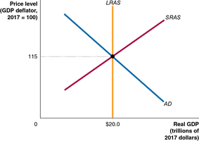
Assume no inflation and growth

Effects of Changes in Aggregate Demand and Supply

• Decrease in AD: Causes recession in the short run; SRAS shifts right over time, restoring equilibrium at a lower price level.

• Increase in AD: Causes expansion and inflation in the short run; SRAS shifts left as wages and prices rise, restoring equilibrium at a higher price level.

• Supply Shock: Sudden shifts in SRAS cause stagflation (recession and inflation); equilibrium is restored as expectations and wages adjust.

• Stagflation, a combination of inflation and recession, usually resulting from a supply shock

Dynamic Aggregate Demand and Aggregate Supply Model

Dynamic Model Features

• Incorporates ongoing growth in real GDP (LRAS shifts right).

• AD and SRAS also shift right over time, except when inflation expectations are high.

• Inflation occurs when AD (total spending) increases faster than LRAS (production)

Macroeconomic Schools of Thought

Key Schools

• Keynesian: Emphasizes sticky wages and prices; government intervention can stabilize the economy.

• Monetarist: Focuses on money supply; advocates a constant monetary growth rule.

• New Classical: Rational expectations; fluctuations minimized by correct expectations and monetary rules.

• Real Business Cycle: Productivity shocks drive business cycles; supply is vertical even in the short run.

• Austrian: Market system superior; business cycles caused by central bank-induced low interest rates.

• Marxist: Critiques capitalism; labor theory of value; predicts eventual transition to communism.

Summary Table: Variables That Shift Aggregate Demand and Supply

Variable	Effect on AD	Effect on SRAS
Monetary Policy	Interest rates ↑ → AD ↓; Interest rates ↓ → AD ↑	No direct effect
Fiscal Policy	Gov. spending ↑ → AD ↑; Taxes ↑ → AD ↓	No direct effect
Expectations	Optimism ↑ → AD ↑; Pessimism ↑ → AD ↓	Higher expected prices → SRAS ↓
Foreign Income	Foreign income ↑ → AD ↑	No direct effect
Exchange Rate	Stronger $ → AD ↓	No direct effect
Labor/Capital	No direct effect	More labor/capital → SRAS ↑
Technology	No direct effect	Improved tech → SRAS ↑
Supply Shock	No direct effect	Input prices ↑ → SRAS ↓

Key Formulas

• Aggregate Demand: $AD = C + I + G + NX$

• GDP (Output): $GDP = C + I + G + NX$

Conclusion

The aggregate demand and aggregate supply model is central to understanding macroeconomic fluctuations, policy impacts, and the business cycle. The chapter also highlights the diversity of macroeconomic schools of thought, each offering unique perspectives on economic dynamics and policy.