Aggregate Demand and Aggregate Supply Analysis – Study Notes

Aggregate Demand and Aggregate Supply Analysis

Introduction

The aggregate demand and aggregate supply (AD-AS) model is a fundamental framework in macroeconomics used to explain short-run fluctuations in real GDP and the price level. This model helps us understand the causes of economic expansions, recessions, and inflation by analyzing the interactions between total demand and total supply in the economy.

Aggregate Demand (AD)

Components of Aggregate Demand

Aggregate demand represents the total quantity of goods and services demanded across all sectors of an economy at various price levels. The four main components are:

• Consumption (C): Spending by households on goods and services.

• Investment (I): Expenditures by firms on capital goods and by households on new housing.

• Government Purchases (G): Spending by government on goods and services.

• Net Exports (NX): Exports minus imports.

The equation for real GDP is:

$Y = C + I + G + NX$

The Aggregate Demand Curve

The aggregate demand curve shows the relationship between the price level and the quantity of real GDP demanded by households, firms, and the government. It slopes downward due to three main effects:

• Wealth Effect: As the price level rises, the real value of household wealth falls, leading to lower consumption.

• Interest-Rate Effect: Higher price levels increase the demand for money, raising interest rates and reducing investment.

• International-Trade Effect: Higher domestic prices make exports more expensive and imports cheaper, reducing net exports.

Implication: Higher price levels lead to lower values of real GDP demanded.

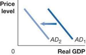
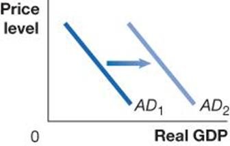
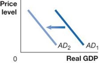
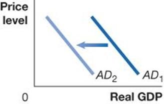
Shifts of the Aggregate Demand Curve

Movements along the AD curve are caused by changes in the price level, holding other factors constant. Shifts in the AD curve occur when a component of real GDP changes due to factors other than the price level.

Variable	Direction of AD Shift	Reason
Interest rates	Left (if increase)	Higher rates raise borrowing costs, reducing C and I
Government purchases	Right (if increase)	Direct component of AD
Personal/business taxes	Left (if increase)	Reduces disposable income and investment
Household/firms' expectations	Right (if optimistic)	Increases C and I
Foreign income/exchange rate	Left (if domestic growth/exchange rate rises)	Reduces net exports

Policy Impacts on Aggregate Demand

• Monetary Policy: The Federal Reserve manages the money supply and interest rates. Raising interest rates decreases investment and shifts AD left; lowering rates increases investment and shifts AD right.

• Fiscal Policy: Changes in government spending and taxation affect AD. Increased government purchases or tax cuts shift AD right; decreased spending or tax hikes shift AD left.

Case Study: The 2020 Recession

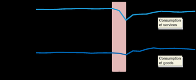
• Consumption: Fell sharply, especially in services.

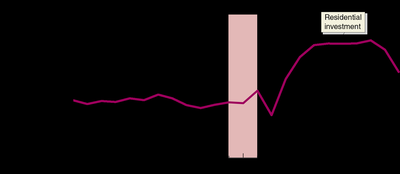
• Investment: Initially fell, but residential investment rebounded due to low interest rates and stimulus.

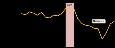
• Net Exports: Decreased, partly due to a stronger dollar and relatively smaller GDP decline in the U.S. compared to trading partners.

Aggregate Supply (AS)

Long-Run Aggregate Supply (LRAS)

The long-run aggregate supply curve shows the relationship between the price level and the quantity of real GDP supplied in the long run. It is vertical because, in the long run, output is determined by resources, technology, and capital—not by the price level. The LRAS is located at the economy's potential or full-employment GDP.

Short-Run Aggregate Supply (SRAS)

The short-run aggregate supply curve is upward sloping. As prices of final goods and services rise, input prices (like wages and raw materials) adjust more slowly, increasing firms' profits and output. Three main reasons for the upward slope are:

• Sticky Wages and Prices: Contracts and slow adjustments make wages and prices inflexible in the short run.

• Slow Wage Adjustments: Firms review wages infrequently and are reluctant to cut wages.

• Menu Costs: The costs of changing prices discourage frequent adjustments.

Shifts of the SRAS Curve

Movements along the SRAS curve are caused by changes in the price level. Shifts occur due to changes in factors other than the price level, such as:

Variable	Direction of SRAS Shift	Reason
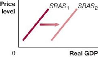
Labor force/capital stock	Right (if increase)	More output can be produced at every price level
Productivity	Right (if increase)	Lower production costs
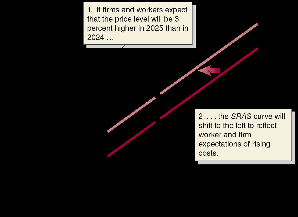
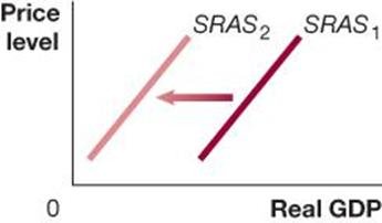
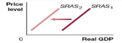
Expected future price level	Left (if increase)	Firms/workers raise wages and prices in anticipation
Adjustment to underestimated prices	Left	Firms/workers catch up to higher price level
Natural resource prices/disasters	Left (if increase)	Higher input costs or reduced supply

Macroeconomic Equilibrium

Short-Run and Long-Run Equilibrium

Macroeconomic equilibrium occurs where the AD and SRAS curves intersect. Long-run equilibrium is achieved when this intersection also occurs at the LRAS, meaning the economy is at full employment.

Effects of Shifts in Aggregate Demand

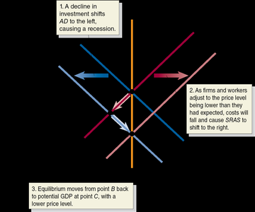
• Decrease in AD: Causes a recession in the short run (output and employment fall). Over time, lower wages and prices shift SRAS right, restoring full employment at a lower price level.

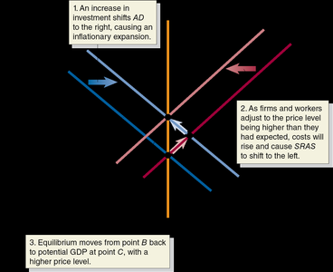
• Increase in AD: Causes an expansion in the short run (output and employment rise, unemployment falls below natural rate). Over time, higher wages and prices shift SRAS left, restoring full employment at a higher price level.

Effects of Supply Shocks

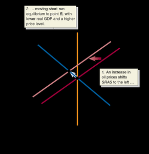
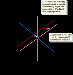
A supply shock (e.g., a sudden increase in oil prices) shifts SRAS left, causing stagflation (higher inflation and lower output). Over time, falling wages and prices shift SRAS right, restoring equilibrium, but the adjustment can take years. Policy intervention can speed recovery but may result in higher prices.

Case Study: The Covid-19 Pandemic

• Both AD and SRAS shifted left due to reduced consumption, investment, and exports, as well as supply disruptions.

• The new equilibrium featured lower real GDP and relatively stable prices.

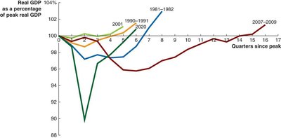
Business Cycle Dynamics

The business cycle is not a regular, predictable cycle. The length and severity of recessions and recoveries vary significantly.

Dynamic Aggregate Demand and Aggregate Supply Model

Incorporating Economic Growth and Inflation

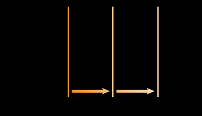
The dynamic AD-AS model accounts for long-run growth and inflation by allowing LRAS, AD, and SRAS to shift over time:

• LRAS: Shifts right as the economy grows (more resources, better technology).

• AD: Typically shifts right due to population growth, technological progress, and policy changes.

• SRAS: Shifts right unless high inflation is expected, which can slow its movement.

Inflation occurs when AD increases faster than LRAS and SRAS.

Understanding Inflation

• When total spending (AD) grows faster than productive capacity (LRAS), the price level rises.

• SRAS may shift right, but if inflation is anticipated, the shift is smaller, leading to higher equilibrium prices.

Main Factors Causing the 2007–2009 Recession

1. End of the housing bubble: Falling house prices reduced residential investment.

2. Financial crisis: Mortgage defaults led to a credit crunch, reducing consumption and investment.

3. Oil price spike: Rising oil prices increased production costs, worsening the recession.

Summary: The AD-AS model is essential for understanding macroeconomic fluctuations, the effects of policy, and the causes of inflation and unemployment. Both demand and supply shocks can have significant short- and long-run effects on output and prices.