Aggregate Demand and Aggregate Supply Analysis: Macroeconomics Chapter 13 Study Notes

Aggregate Demand and Aggregate Supply Analysis

Introduction

This chapter explores the aggregate demand and aggregate supply (AD-AS) model, a fundamental framework in macroeconomics for understanding short-run fluctuations in real GDP and the price level. The chapter also discusses macroeconomic equilibrium, the dynamic AD-AS model, and various schools of macroeconomic thought.

Aggregate Demand

Definition and Components

Aggregate demand (AD) represents the total quantity of goods and services demanded across all levels of an economy at a given overall price level and in a given period. The four main components of real GDP are:

• Consumption (C): Spending by households on goods and services.

• Investment (I): Spending by firms on capital goods and by households on new housing.

• Government Purchases (G): Spending by governments on goods and services.

• Net Exports (NX): Exports minus imports.

The aggregate demand equation is:

$Y = C + I + G + NX$

The Aggregate Demand Curve

The AD curve shows the relationship between the price level and the quantity of real GDP demanded by households, firms, and the government. It slopes downward due to three main effects:

• Wealth Effect: As the price level rises, the real value of household wealth falls, leading to lower consumption.

• Interest-Rate Effect: Higher price levels increase the demand for money, raising interest rates and reducing investment.

• International-Trade Effect: Higher domestic prices make exports more expensive and imports cheaper, reducing net exports.

Movements vs. Shifts of the AD Curve

• Movement along the AD curve: Caused by a change in the price level, holding all else constant.

• Shift of the AD curve: Caused by changes in components of GDP other than the price level (e.g., changes in government purchases, taxes, expectations, foreign income, or exchange rates).

Determinants of Aggregate Demand

Variable	Direction of Shift	Reason
Interest rates	Left (if increase)	Higher rates reduce consumption and investment
Government purchases	Right (if increase)	Direct component of AD
Personal/business taxes	Left (if increase)	Reduces disposable income and investment
Household expectations	Right (if optimistic)	Increases consumption and investment
Firms' expectations	Right (if optimistic)	Increases investment
Foreign income	Left (if domestic grows faster)	Imports rise faster than exports
Exchange rate	Left (if domestic currency appreciates)	Exports fall, imports rise

Policy Impacts

• Monetary Policy: The Federal Reserve manages the money supply and interest rates. Higher interest rates reduce AD; lower rates increase AD.

• Fiscal Policy: Changes in government spending and taxation affect AD directly through G and indirectly through C and I.

Recent Example: The 2020 Recession

• Consumption spending fell, especially on services.

• Residential investment increased later due to low interest rates and stimulus.

• Net exports decreased due to a stronger dollar and relatively smaller GDP decline in the U.S. compared to trading partners.

Aggregate Supply

Definition and Types

Aggregate supply (AS) is the total quantity of goods and services that firms are willing and able to supply at different price levels. The relationship between output and price level differs in the short run and long run:

• Long-Run Aggregate Supply (LRAS): Vertical at the level of potential or full-employment GDP, determined by resources, technology, and capital stock. Not affected by the price level.

• Short-Run Aggregate Supply (SRAS): Upward sloping because input prices adjust more slowly than output prices, and due to wage and price stickiness.

Why the SRAS Curve Is Upward Sloping

• Sticky Wages and Prices: Contracts and slow adjustments make wages and prices inflexible in the short run.

• Slow Wage Adjustments: Firms review wages infrequently and dislike wage cuts.

• Menu Costs: The costs of changing prices discourage frequent adjustments.

Movements vs. Shifts of the SRAS Curve

• Movement along SRAS: Caused by a change in the price level, holding other factors constant.

• Shift of SRAS: Caused by changes in factors such as labor force, capital stock, productivity, expected future prices, and input prices.

Determinants of Short-Run Aggregate Supply

Variable	Direction of Shift	Reason
Labor force/capital stock	Right (if increase)	More output at every price level
Productivity	Right (if increase)	Lower production costs
Expected future price level	Left (if increase)	Firms/workers raise wages and prices
Adjustment to underestimated prices	Left	Firms/workers catch up to higher prices
Natural resource prices/disasters	Left (if increase)	Higher costs or reduced supply

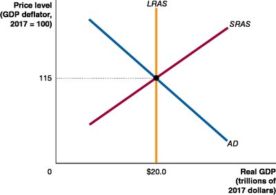
Macroeconomic Equilibrium

Short-Run and Long-Run Equilibrium

Equilibrium occurs where the AD and SRAS curves intersect. Long-run equilibrium is achieved when this intersection also occurs at the LRAS, meaning the economy is at full employment.

Adjustment to Shocks

• Decrease in AD: Causes a recession in the short run. Over time, lower wages and prices shift SRAS right, restoring long-run equilibrium at a lower price level.

• Increase in AD: Causes an expansion in the short run. Higher wages and prices shift SRAS left, restoring long-run equilibrium at a higher price level.

• Supply Shock: A sudden leftward shift in SRAS (e.g., oil price spike) causes stagflation (recession + inflation). Over time, lower wages and prices can shift SRAS back right.

Case Study: The Covid-19 Pandemic

• Both AD and SRAS shifted left due to reduced consumption, investment, and exports, as well as supply disruptions.

• Resulted in lower real GDP and relatively stable prices in the short run.

Dynamic Aggregate Demand and Aggregate Supply Model

Incorporating Growth and Inflation

The dynamic AD-AS model accounts for ongoing economic growth and inflation:

• LRAS shifts right over time as the economy grows.

• AD typically shifts right due to population growth, technological progress, and policy.

• SRAS also shifts right, except when inflation expectations rise.

Understanding Inflation

• Inflation occurs when AD increases faster than LRAS.

• SRAS shifts right, but less than LRAS if inflation is anticipated, leading to a higher price level in long-run equilibrium.

Case Study: The 2007–2009 Recession

• Caused by the end of the housing bubble, a financial crisis, and a rapid increase in oil prices (supply shock).

• Resulted in lower real GDP and higher prices relative to potential GDP.

Appendix: Macroeconomic Schools of Thought

Key Schools of Thought

• Keynesian: Emphasizes the role of aggregate demand and sticky wages/prices in causing economic fluctuations. Advocates for active government policy.

• New Keynesian: Builds on Keynes by emphasizing wage and price stickiness.

• Monetarist: Focuses on the money supply as the main driver of economic fluctuations. Advocates for a constant growth rate of money supply.

• New Classical: Emphasizes rational expectations and the importance of correct price level expectations.

• Real Business Cycle: Attributes business cycles to real (not monetary) shocks, such as productivity changes. Assumes quick adjustment of prices and wages.

• Austrian: Argues that central bank-induced low interest rates cause business cycles through overinvestment.

• Karl Marx: Criticized capitalism, predicting its eventual replacement by communism due to worker exploitation.

Note: There is no consensus on which school is correct; evidence can often be interpreted in multiple ways.

Summary Table: Factors Shifting AD and SRAS

Factor	AD Shift	SRAS Shift
Interest rates	Left (if increase)	—
Government purchases	Right (if increase)	—
Taxes	Left (if increase)	—
Expectations (households/firms)	Right (if optimistic)	Left (if expect higher prices)
Foreign income/exchange rate	Left (if domestic grows faster or currency appreciates)	—
Labor force/capital stock	—	Right (if increase)
Productivity	—	Right (if increase)
Input prices/disasters	—	Left (if increase)

Additional info: This summary includes expanded academic context and examples for clarity and exam preparation.