Aggregate Demand and Aggregate Supply: Core Concepts and Policy Implications

Aggregate Demand and Aggregate Supply Analysis

Aggregate Demand (AD)

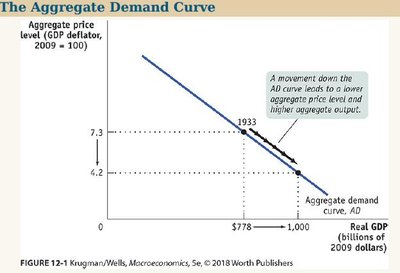
The Aggregate Demand (AD) curve illustrates the relationship between the overall price level in an economy and the total quantity of goods and services demanded by households, firms, the government, and foreign buyers. The AD curve is typically downward sloping, reflecting the inverse relationship between the price level and real GDP demanded.

• Wealth Effect: As the price level rises, the real value of money holdings falls, reducing consumers' purchasing power and thus decreasing the quantity of goods and services demanded.

• Interest Rate Effect: Higher price levels lead to higher interest rates, which reduce investment and consumption.

• International Trade Effect: As domestic prices rise, exports become more expensive and imports become relatively cheaper, reducing net exports.

Movements vs. Shifts of the AD Curve

• Movement along the AD curve: Caused by a change in the aggregate price level, leading to a change in the quantity of aggregate output demanded.

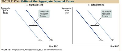
• Shift of the AD curve: Occurs when factors other than the price level change, such as changes in expectations, wealth, fiscal policy (government spending or taxes), or monetary policy.

Aggregate Supply (AS)

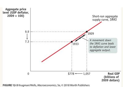
The Aggregate Supply (AS) curve shows the relationship between the overall price level and the quantity of goods and services that firms are willing to produce. In the short run, the AS curve is upward sloping due to sticky wages and prices, meaning that as the price level rises, firms are willing to supply more output.

• Short-Run Aggregate Supply (SRAS): Positively sloped because some input costs (especially wages) are fixed in the short run, so higher prices increase profits and output.

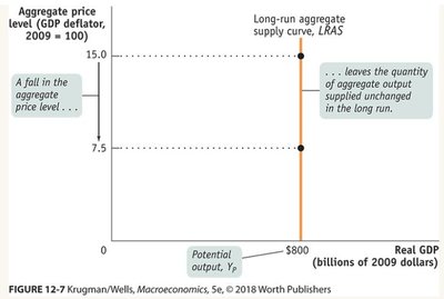
• Long-Run Aggregate Supply (LRAS): Vertical at the economy's potential output (YPOT), reflecting that in the long run, all prices and wages are flexible and output is determined by resources and technology, not the price level.

Movements vs. Shifts of the AS Curve

• Movement along the AS curve: Caused by a change in the aggregate price level.

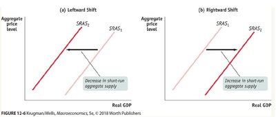
• Shift of the AS curve: Caused by changes in input prices (e.g., oil prices), productivity, or other factors affecting production costs.

Long-Run Aggregate Supply (LRAS) and Potential Output

The LRAS curve is vertical at the level of potential output (YPOT), which is the maximum sustainable output an economy can produce when all resources are fully employed. Changes in the price level do not affect potential output in the long run.

Business Cycle and Potential Output

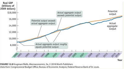
Actual GDP fluctuates around potential output due to business cycles. During expansions, actual output may exceed potential output; during recessions, it may fall below.

From Short Run to Long Run: Wage Adjustment and Self-Correction

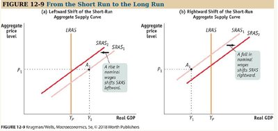
In the short run, output can deviate from potential due to sticky wages and prices. Over time, wage and price adjustments return the economy to potential output:

• Above potential output: Wages rise, shifting SRAS leftward, reducing output back to potential.

• Below potential output: Wages fall, shifting SRAS rightward, increasing output back to potential.

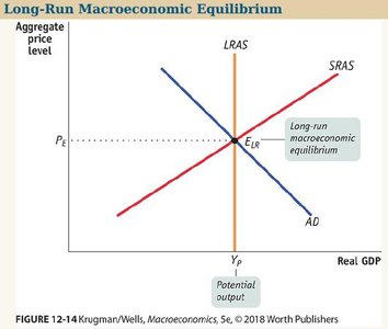
The AD-AS Model: Macroeconomic Equilibrium

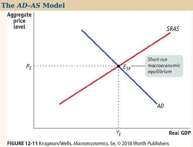
The intersection of the AD and AS curves determines the short-run macroeconomic equilibrium, with a specific price level and real GDP. In the long run, the economy tends to return to the intersection of AD, SRAS, and LRAS at potential output.

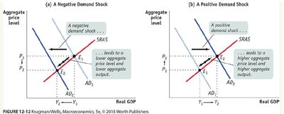
Demand and Supply Shocks

• Demand Shock: An event that shifts the AD curve (e.g., changes in consumer confidence, government spending, or taxes).

• Supply Shock: An event that shifts the AS curve (e.g., changes in oil prices, technological advances, or wage changes).

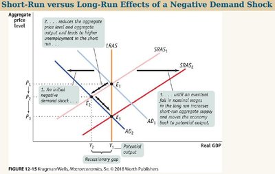
Short-Run vs. Long-Run Effects of Shocks

• Negative demand shock: Initially reduces output and price level; over time, falling wages shift SRAS right, restoring output but at a lower price level.

• Positive demand shock: Initially increases output and price level; over time, rising wages shift SRAS left, restoring output but at a higher price level.

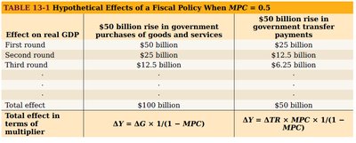
Fiscal Policy and the Multiplier

Fiscal policy refers to government decisions on spending and taxation to influence aggregate demand. The multiplier effect describes how an initial change in spending leads to a larger change in GDP.

• Government purchases multiplier: $\Delta Y = \Delta G \times \frac{1}{1 - MPC}$

• Tax multiplier: $\Delta Y = \Delta T \times \frac{MPC}{1 - MPC}$

• MPC (Marginal Propensity to Consume): The fraction of additional income that households spend on consumption.

Effect on real GDP	$50 billion rise in government purchases of goods and services	$50 billion rise in government transfer payments
First round	$50 billion	$25 billion
Second round	$25 billion	$12.5 billion
Third round	$12.5 billion	$6.25 billion
Total effect	$100 billion	$50 billion
Total effect in terms of multiplier	$\Delta Y = \Delta G \times \frac{1}{1 - MPC}$	$\Delta Y = \Delta TR \times MPC \times \frac{1}{1 - MPC}$

Budget Deficits and Public Debt

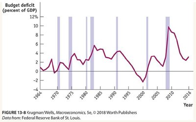
Budget deficit: The amount by which government spending exceeds government revenue in a given year. Public debt is the accumulation of past deficits.

• Deficits are common during recessions due to expansionary fiscal policy.

• Surpluses are rare and typically occur during economic booms.

• Automatic stabilizers (e.g., taxes and transfers) help smooth the business cycle by increasing deficits in recessions and reducing them in booms.

Debt Sustainability

To assess whether a government's debt is sustainable, compare the growth rate of GDP (g) to the interest rate on government bonds (r). If g > r, governments can run small deficits indefinitely without increasing the debt-to-GDP ratio.

• Debt-to-GDP ratio: $b_t = \frac{B_t}{Y_t}$

• Stabilizing condition: $s_{t+1} = (r - g) b$

If the interest rate exceeds the growth rate, a primary surplus is needed to stabilize the debt ratio.

Policy Debates: Hawks vs. Doves

• Hawks: Prioritize low inflation, cautious about fiscal expansion, support central bank independence.

• Doves: Prioritize GDP growth, favor expansionary fiscal policy, optimistic about government investment efficiency.

Summary Table: Key Concepts in AD-AS Analysis

Concept	Definition	Key Equation
Aggregate Demand (AD)	Total quantity of goods/services demanded at different price levels	AD = C + I + G + (EX - IM)
Aggregate Supply (AS)	Total quantity of goods/services supplied at different price levels	SRAS: upward sloping; LRAS: vertical at YPOT
Multiplier	Amplification of initial spending change on GDP	$\frac{1}{1 - MPC}$
Budget Deficit	G - T (when G > T)	SGOV = T - G - TR
Debt Sustainability	Stable debt-to-GDP ratio	$s_{t+1} = (r - g) b$

Additional info: This summary integrates textbook diagrams and equations to provide a comprehensive, exam-ready overview of the AD-AS model, fiscal policy, and macroeconomic equilibrium.