Aggregate Demand and Aggregate Supply: Macroeconomic Equilibrium and Policy Implications

Aggregate Demand and Aggregate Supply Analysis

Introduction to the Aggregate Demand and Aggregate Supply Model

The aggregate demand and aggregate supply (AD-AS) model is a fundamental framework in macroeconomics used to explain short-run fluctuations in real GDP and the price level. The intersection of the aggregate demand curve and the short-run aggregate supply curve determines the equilibrium level of real GDP and the price level in the economy.

• Real GDP is measured on the horizontal axis.

• Price level is measured on the vertical axis, typically using the GDP deflator.

• Equilibrium occurs where AD and SRAS intersect.

Aggregate Demand

Definition and Slope of the Aggregate Demand Curve

The aggregate demand (AD) curve shows the total quantity of goods and services demanded across all levels of price. The AD curve slopes downward due to three main effects:

• Wealth Effect: As the price level rises, the purchasing power of financial assets falls, reducing consumption.

• Interest Rate Effect: Higher price levels lead to higher interest rates, which dampen investment spending.

• Export Effect: When domestic prices rise relative to foreign prices, exports decrease as domestic goods become more expensive abroad.

Determinants and Shifts of Aggregate Demand

Factors that shift the AD curve include changes in the components of GDP:

• Government spending or taxes

• Household spending: Influenced by income, wealth, and consumer confidence

• Firm spending: Affected by interest rates and business expectations

• Foreign variables: Exchange rates and foreign demand for domestic goods

A rightward shift indicates an increase in aggregate demand, while a leftward shift indicates a decrease.

Movements Along vs. Shifts of the Aggregate Demand Curve

A movement along the AD curve is caused by a change in the price level, holding all else constant. A shift of the AD curve is caused by changes in non-price determinants, such as fiscal policy or changes in consumer confidence.

Components of Aggregate Demand

• Consumer Spending: Driven by wealth, confidence, debt, and taxes. For example, a stock market boom can increase consumer spending via the wealth effect.

• Investment: Determined by interest rates and expected returns. Higher interest rates reduce investment and shift AD left; improved business expectations increase investment and shift AD right.

• Government Spending: Increases in government spending shift AD right; decreases shift it left.

• Exports: Higher foreign income or favorable exchange rates increase exports and shift AD right.

Examples of Changes in Aggregate Demand

• Tax cuts by Congress: Increase AD

• Decrease in investment spending: Decrease AD

• Increase in government spending with no tax increase: Increase AD

• Jump in consumer confidence: Increase AD

• Stock market collapse: Decrease AD

Aggregate Supply

Definition and Shapes of the Aggregate Supply Curve

The aggregate supply (AS) curve shows the total quantity of goods and services that firms are willing to produce at different price levels. There are two main forms:

• Short-Run Aggregate Supply (SRAS): Upward sloping due to sticky input costs (e.g., wages, rents).

• Long-Run Aggregate Supply (LRAS): Vertical at the economy's potential output, representing full employment.

Short-Run Aggregate Supply

SRAS is upward sloping because input costs are slow to adjust. As prices rise, firms' profits increase, leading to higher output. However, as production expands, input costs eventually rise, limiting further output increases.

Determinants and Shifts of Aggregate Supply

Variables that shift the SRAS curve include:

• Changes in labor productivity

• Changes in average wage rates

• Technological changes

• Changes in capital stock

• Expectations of future price levels

• Changes in the price of important natural resources

Rising productivity or technological advances shift SRAS right; higher input costs shift it left.

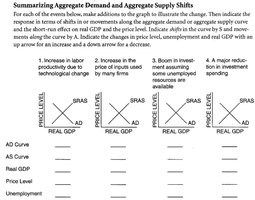
Examples of Changes in Aggregate Supply

• Increase in wage rates: Decrease SRAS

• Increase in oil prices: Decrease SRAS

• Increase in labor productivity: Increase SRAS

• Discovery of new energy resources: Increase SRAS

• Technological improvements: Increase SRAS

Long-Run Aggregate Supply

Definition and Economic Growth

The long-run aggregate supply (LRAS) curve is vertical, indicating that in the long run, the economy's output is determined by resources, technology, and institutions, not by the price level. LRAS represents full employment and is analogous to the production possibilities frontier.

• An outward shift in LRAS indicates economic growth.

Macroeconomic Equilibrium

Short-Run and Long-Run Equilibrium

Equilibrium occurs where AD, SRAS, and LRAS intersect. In the short run, shifts in AD or SRAS can cause recessions or expansions. In the long run, the economy returns to potential output, with price level adjustments.

• Recession: Short-run decrease in AD reduces output and increases unemployment; in the long run, prices adjust downward, restoring full employment.

• Expansion: Short-run increase in AD raises output and prices; in the long run, only the price level remains higher.

Demand-Pull and Cost-Push Inflation

• Demand-Pull Inflation: Occurs when AD increases beyond full employment, causing upward pressure on prices.

• Cost-Push Inflation: Caused by supply shocks (e.g., oil price spikes) that shift SRAS left, raising prices and reducing output.

Stagflation

Stagflation is a combination of inflation and recession, typically resulting from a supply shock. It is characterized by rising prices and falling output.

Case Study: The 2007–2009 Recession

The 2007–2009 recession was marked by large declines in aggregate demand, especially in housing investment. Financial crises tend to cause deeper and longer-lasting declines in AD compared to other shocks.

Wages and Prices during Recessions

During recessions, firms are generally reluctant to cut wages due to concerns about worker morale and productivity. Price levels rarely fall for an entire year in the U.S., even during severe recessions. Wage and price stickiness help explain why recessions can persist.

Appendix: Macroeconomic Schools of Thought

Keynesian Revolution

The Keynesian model emphasizes the role of aggregate demand in determining output and employment, especially in the short run.

The Monetarist Model

Monetarism, associated with Milton Friedman, argues that the money supply should grow at a constant rate. The monetarist model (neo-Quantity Theory of Money) stresses the importance of monetary policy in controlling inflation.

The New Classical Model

New classical macroeconomics (Robert Lucas and others) emphasizes rational expectations and the idea that markets clear quickly, making policy interventions less effective.

Karl Marx: Capitalism’s Severest Critic

Karl Marx argued that capitalism would eventually be replaced by communism due to inherent exploitation of workers. He believed in the labor theory of value and predicted that monopolization would impoverish the masses. However, Marx did not provide a detailed blueprint for a communist economy, and few countries today claim to follow his ideas.

Key Equations

• Aggregate Demand (AD): $AD = C + I + G + (X - M)$

• Short-Run Aggregate Supply (SRAS): $Y = Y^* + \alpha (P - P^e)$ (where $Y$ is output, $Y^*$ is potential output, $P$ is the price level, $P^e$ is the expected price level, and $\alpha$ is a positive parameter)

Additional info: The equations above summarize the main relationships in the AD-AS model. The AD equation shows the components of aggregate demand, while the SRAS equation illustrates how output deviates from potential when actual and expected prices differ.