Aggregate Demand and Aggregate Supply: Short-Run Economic Fluctuations

Aggregate Demand and Aggregate Supply

Introduction to Short-Run Economic Fluctuations

Macroeconomic activity does not follow a smooth, predictable path but instead fluctuates over time. These short-run fluctuations, known as business cycles, are explained using the model of aggregate demand (AD) and aggregate supply (AS). This model helps us understand how changes in total spending and production can lead to recessions or expansions, and how policy can influence these outcomes.

Key Facts about Short-Run Economic Fluctuations

Business Cycles and Economic Variables

• Recession: A period of declining real incomes and rising unemployment.

• Depression: A severe recession.

• Irregularity: Economic fluctuations are unpredictable and irregular.

• Co-movement: Most macroeconomic variables (GDP, spending, investment, etc.) fluctuate together, though by different amounts.

• Output and Unemployment: As output falls, unemployment rises.

• Example: During the 2008–2009 recession, Canadian real GDP fell by 3% and unemployment rose significantly.

Short Run vs. Long Run in Macroeconomics

Classical Theory and Its Limitations

• Classical Theory: In the long run, money is neutral and only real variables (output, employment) matter.

• Short Run: Real and nominal variables are intertwined; changes in the money supply can affect real output and employment.

• Need for a New Model: The AD-AS model is used to analyze short-run fluctuations where classical assumptions do not hold.

The Aggregate Demand (AD) Curve

Definition and Components

The aggregate demand curve shows the total quantity of goods and services demanded across all sectors (households, firms, government, and foreign buyers) at each price level. It is downward sloping, indicating an inverse relationship between the price level and the quantity of output demanded.

• Formula: $Y = C + I + G + NX$ where $Y$ is GDP, $C$ is consumption, $I$ is investment, $G$ is government purchases, and $NX$ is net exports.

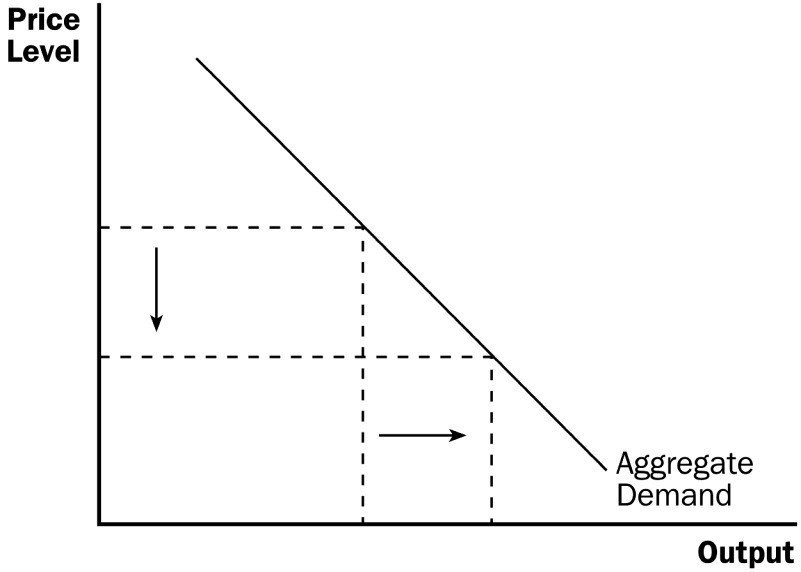
Why the AD Curve Slopes Downward

• Wealth Effect: Lower price levels increase the real value of money, making consumers feel wealthier and increasing consumption.

• Interest Rate Effect: Lower price levels reduce the demand for money, lowering interest rates and stimulating investment.

• Exchange Rate Effect: Lower price levels decrease the real exchange rate, making domestic goods cheaper for foreigners, increasing exports.

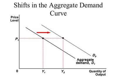
Shifts in the Aggregate Demand Curve

The AD curve shifts when there are changes in consumption, investment, government purchases, or net exports, independent of the price level.

• Consumption: Increased consumer confidence or tax cuts shift AD right; increased saving shifts AD left.

• Investment: Technological advances, business optimism, or lower interest rates shift AD right; expiration of investment tax credits shifts AD left.

• Government Purchases: Increased government spending shifts AD right; spending cuts shift AD left.

• Net Exports: Foreign recessions or a stronger domestic currency shift AD left; a weaker currency or foreign booms shift AD right.

The Aggregate Supply (AS) Curve

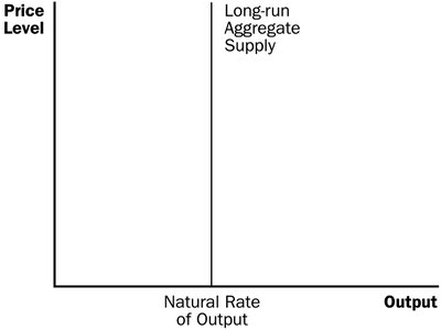
Long-Run Aggregate Supply (LRAS)

In the long run, aggregate supply is determined by the economy’s resources and technology, not by the price level. The LRAS curve is vertical at the natural rate of output (potential output), where unemployment is at its natural rate.

• Production Function: $Y = A F(L, K, H, N)$ where $Y$ is output, $A$ is technology, $L$ is labor, $K$ is capital, $H$ is human capital, $N$ is natural resources.

• Shifts in LRAS: Caused by changes in labor, capital, natural resources, or technology.

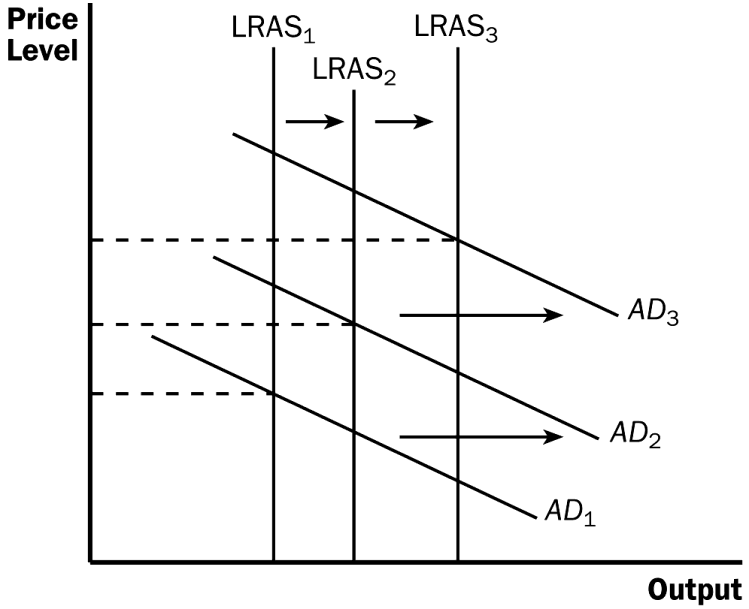
Long-Run Growth and Inflation

Technological progress shifts LRAS right, while monetary policy can shift AD. Over time, this leads to economic growth and inflation.

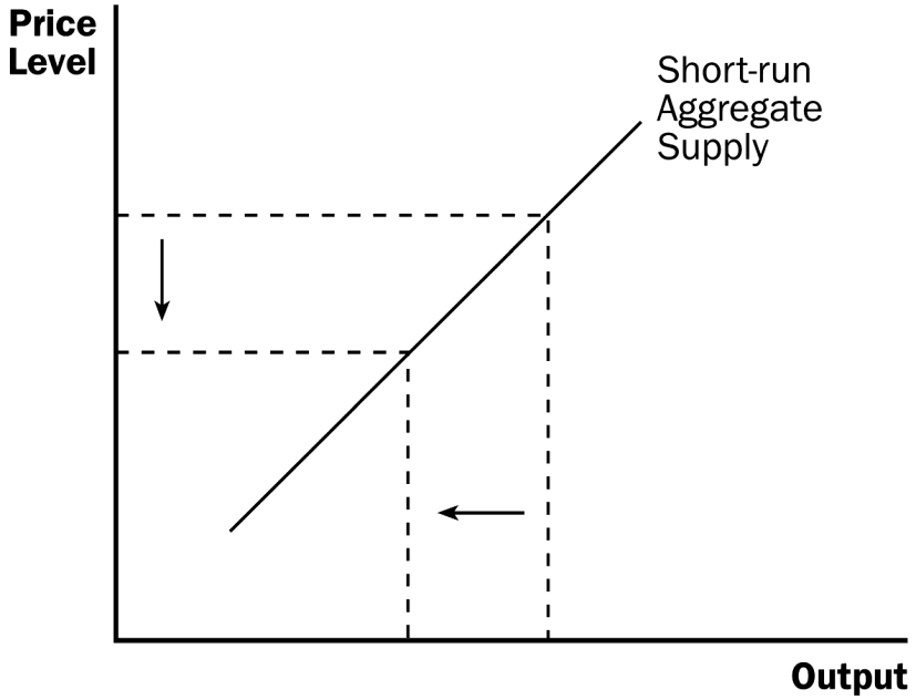
Short-Run Aggregate Supply (SRAS)

In the short run, the AS curve is upward sloping. This means that as the price level rises, firms are willing to produce more output due to sticky wages, sticky prices, and misperceptions about relative prices.

• Sticky-Wage Theory: Nominal wages are slow to adjust, so unexpected changes in prices affect real wages and production.

• Sticky-Price Theory: Some prices are slow to adjust due to menu costs, causing output to respond to price changes.

• Misperceptions Theory: Producers may misinterpret changes in the overall price level as changes in relative prices, affecting output decisions.

• SRAS Equation: $Y = Y_N + \alpha (P - P_E)$ where $Y$ is output, $Y_N$ is natural rate of output, $P$ is actual price level, $P_E$ is expected price level, $\alpha$ is a positive parameter.

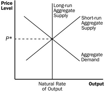
Macroeconomic Equilibrium

Long-Run and Short-Run Equilibrium

Equilibrium occurs where AD intersects both SRAS and LRAS. In the long run, output returns to its natural rate, but in the short run, output and prices can deviate due to shocks.

Economic Fluctuations: Shifts in AD and AS

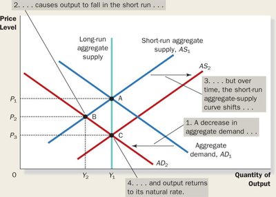
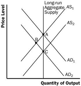
Shifts in Aggregate Demand

• A leftward shift in AD (e.g., due to pessimism or reduced wealth) causes output and prices to fall in the short run. Over time, SRAS shifts right as wages and prices adjust, restoring output to its natural rate but at a lower price level.

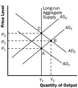
Shifts in Aggregate Supply

• An adverse shift in SRAS (e.g., due to higher production costs) causes stagflation: output falls and prices rise. Over time, lower output puts downward pressure on wages, shifting SRAS back to the right and restoring output to its natural rate.

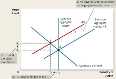
Stagflation

• Stagflation: A period of falling output and rising prices, typically caused by a leftward shift in SRAS.

Practice and Application

Example Scenarios

• Stock Market Decline: AD shifts left; output and price level fall in the short run, but output returns to natural rate in the long run as SRAS shifts right.

• Government Spending Increase: AD shifts right; output and price level rise in the short run, but only price level remains higher in the long run.

• Technological Improvement: Both LRAS and SRAS shift right; output rises and price level falls.

• Foreign Recession: AD shifts left; output and price level fall in the short run, output returns to natural rate in the long run.

Summary Table: Effects of Shocks in the AD-AS Model

Shock	Short-Run Effect	Long-Run Effect
AD shifts left	Output ↓, Price Level ↓	Output returns to natural rate, Price Level ↓
AD shifts right	Output ↑, Price Level ↑	Output returns to natural rate, Price Level ↑
SRAS shifts left	Output ↓, Price Level ↑ (stagflation)	Output returns to natural rate, Price Level returns to initial
SRAS shifts right	Output ↑, Price Level ↓	Output returns to natural rate, Price Level returns to initial

Key Terms

• Aggregate Demand (AD): Total quantity of goods and services demanded at each price level.

• Aggregate Supply (AS): Total quantity of goods and services supplied at each price level.

• Long-Run Aggregate Supply (LRAS): Vertical at the natural rate of output.

• Short-Run Aggregate Supply (SRAS): Upward sloping due to sticky wages, sticky prices, and misperceptions.

• Stagflation: Combination of recession and inflation.

• Natural Rate of Output: Output when unemployment is at its natural rate.