Aggregate Demand and Supply: Gaps, Adjustments, and Fiscal Policy

Aggregate Demand and Aggregate Supply Model

Overview of the AD-AS Model

The Aggregate Demand (AD) and Aggregate Supply (AS) model is a central framework in macroeconomics for analyzing fluctuations in real GDP, employment, and the price level. It helps explain short-run economic cycles and long-run growth.

• Aggregate Demand (AD): Represents the total demand for goods and services in an economy at different price levels.

• Aggregate Supply (AS): Shows the total output firms are willing to produce at various price levels.

• Short-Run vs. Long-Run: In the short run, prices and wages may be sticky, while in the long run, they adjust fully.

Example: A sudden increase in consumer confidence can shift the AD curve to the right, increasing output and price level in the short run.

Macroeconomic Gaps: Recessionary and Inflationary

Recessionary Gap

A recessionary gap occurs when actual real GDP is below potential GDP (Y*), indicating underutilized resources and higher unemployment.

• Causes: Decline in aggregate demand due to reduced consumption, investment, government spending, or net exports.

• Adjustment Mechanisms:

  • Falling wages and factor prices shift the short-run aggregate supply (SRAS) curve to the right, restoring equilibrium at potential GDP.

  • Expansionary fiscal policy (increased government spending or tax cuts) shifts the AD curve to the right.

Example: During a recession, governments may increase spending to boost aggregate demand.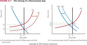

Inflationary Gap

An inflationary gap arises when actual real GDP exceeds potential GDP, leading to upward pressure on prices and lower unemployment.

• Causes: Excessive aggregate demand from high consumption, investment, or government spending.

• Adjustment Mechanisms:

  • Rising wages and factor prices shift the SRAS curve to the left, reducing output to potential GDP.

  • Contractionary fiscal policy (decreased government spending or increased taxes) shifts the AD curve to the left.

Example: If the economy overheats, the government may raise taxes to cool demand.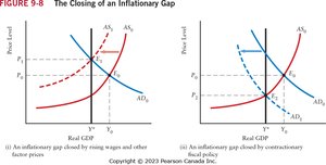

Shifts and Movements in Aggregate Demand and Supply

Shifts of the AD Curve

The AD curve shifts due to changes in its components:

• Consumption (C)

• Investment (I)

• Government Spending (G)

• Net Exports (NX)

Formula: $AD = C + I + G + NX$

• An increase in any component shifts AD right; a decrease shifts it left.

Why the AD Curve is Downward Sloping

• Wealth Effect: Higher price levels reduce real wealth, lowering consumption.

• Interest Rate Effect: Higher prices increase interest rates, reducing investment.

• Net Export Effect: Higher domestic prices make exports less competitive, reducing net exports.

Shifts of the SRAS Curve

The SRAS curve shifts due to changes in input costs, productivity, and expectations.

• Increase in Labour Force: Shifts SRAS right.

• Improved Productivity: Shifts SRAS right.

• Supply Shocks: Negative shocks (e.g., oil price spike) shift SRAS left.

Why the SRAS Curve is Upward Sloping

• Sticky Wages and Prices: Contracts and menu costs prevent immediate adjustment.

• Slow Wage Adjustment: Firms are slow to change wages in response to economic conditions.

• Difficulty Predicting Prices: Uncertainty leads to gradual adjustments.

Long-Run Macroeconomic Equilibrium

Adjustment to Full Potential

In the long run, the economy returns to potential GDP (Y*) as wages and prices fully adjust.

• Self-Correcting Mechanism: Recessionary gaps close as wages fall; inflationary gaps close as wages rise.

• Role of Expectations: If workers expect higher future prices, they demand higher wages, shifting SRAS left.

Fiscal Policy and Economic Stabilization

Automatic Stabilizers

Automatic stabilizers are fiscal mechanisms that counteract economic fluctuations without new government action.

• Progressive Taxation: Taxes rise with income, dampening booms.

• Transfers: Unemployment benefits rise during recessions, supporting demand.

• Multiplier Effect: Taxes and transfers reduce the size of the multiplier, moderating swings.

Discretionary Fiscal Policy

Discretionary fiscal policy involves deliberate changes in government spending or taxation to close output gaps.

• Closing a Recessionary Gap: Increase spending or cut taxes.

• Closing an Inflationary Gap: Decrease spending or raise taxes.

Phillips Curve and Tradeoffs

Unemployment and Inflation

The Phillips Curve illustrates the short-run tradeoff between unemployment and inflation.

• Lower Unemployment: Often associated with higher inflation.

• Higher Unemployment: Often associated with lower inflation.

Supply Side and Economic Growth

Factors Driving Growth

• Labour Force Growth: Increases productive capacity.

• Technological Progress: Shifts LRAS right, raising potential GDP.

Static vs. Dynamic AD-AS Models

Dynamic Model Features

• Increasing Real GDP: LRAS shifts right over time.

• AD Shifts: Typically rightward due to population and productivity growth.

• SRAS Shifts: Rightward except when inflation expectations are high.

Saving Paradox

Short-Run vs. Long-Run Effects

• Short Run: Increased saving reduces consumption and GDP.

• Long Run: Higher saving boosts investment and future GDP.

Example: If households suddenly save more, the economy may slow initially but grow faster in the future. Additional info: These notes expand on brief points with academic context, definitions, and examples for clarity.